A Horn Antenna
In this example, we showcase a validated HFWorks simulation of a high-efficiency horn antenna designed to illuminate a passive parabolic reflector. The original design utilizes two waves with distinct modes, resulting in a remarkably clean radiation pattern. For validation, we simulate the model with a single wave to assess return loss matching. Additionally, we present results pertaining to radiation patterns and the distribution of the inner electric field.
![The feed with parabolic reflector used for sun noise measurement [1]](/ckfinder/userfiles/images/image001.png)
Figure 1 - The feed with a parabolic reflector used for sun noise measurement [1]
![antenna side view (left) and probe (right) dimensions [1]](/ckfinder/userfiles/images/image002(3).jpg)
![antenna side view (left) and probe (right) dimensions [1]](/ckfinder/userfiles/images/image003.png)
Figure 2 - antenna side view (left) and probe (right) dimensions [1]
![antenna 3D SolidWorks views (regular and transparent) [1]](/ckfinder/userfiles/images/image004(5).jpg)
![antenna 3D SolidWorks views (regular and transparent) [1]](/ckfinder/userfiles/images/image005(3).jpg)
Figure 3 - antenna 3D views (regular and transparent) [1]
The mesh is refined, especially around the coaxial probe. HFWorks offers a default mesh that intelligently adapts to the structure's dimensions. However, users have complete control over the global mesh size and can apply mesh controls to areas of greater relevance. It's crucial to ensure that mesh elements do not exceed one-tenth of the free space wavelength for optimal results. A 3D mesh model's colored chart allows a detailed examination of the mesh in inner regions. The structure underwent discretization into a finite element mesh, and the analysis was carried out using the antenna solver.
.jpg)
Figure 4 - Mesh of the structure
Simulation
Solids and Materials
We apply the port to the circular surface of the coax and check the Pure TEM check box. We signal that the septum is a PEC. The feed horn is filled with air but its surfaces are treated as PEC.
Results
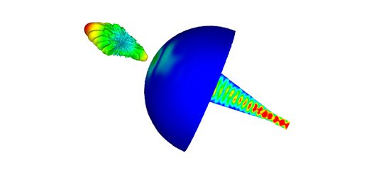
Once the model is meshed and analyzed, we can examine the electric field distribution. This can be visualized in both fringe and vector formats, with the option to animate the field. Section clipping views can also be employed to observe the distribution within inner regions of the structure.
.jpg)
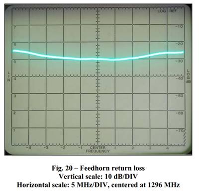
The return loss plot, displayed in this graph spanning from 1.1 GHz to 1.5 GHz, reveals a minimum point at around 1.29 GHz. To enhance accuracy, we can conduct an additional study within the range of 1.25 GHz to 1.32 GHz, as depicted in the subsequent figure.
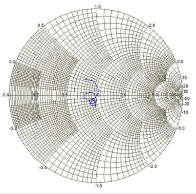
Figure 5 - Return loss curves. (Smith Chart from 1.1 to 1.5 GHz)
![Measurement results from [1] along side HFWorks' simulation results](/ckfinder/userfiles/images/image009.jpg)
Figure 6 - Measurement results from [1] alongside HFWorks' simulation results
For radiation pattern visualization, the electrical parameters folder provides two types of polar plots (2D and 3D). Users can select the preferred type and choose from various variables to plot. Typically, we opt for the Total Electric Field to display the antenna's radiation pattern. Additionally, there are alternative options like different electric field components, antenna gain, axial ratio, and more. The following figure illustrates the antenna's radiation pattern, demonstrating excellent agreement with the measurements in [1].
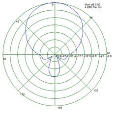
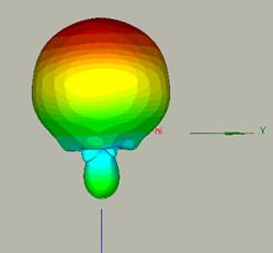
Figure 7 - Radiation patterns at 1.296 GHz simulated in HFWorks.
Conclusion
This application note demonstrates a high-efficiency horn antenna designed to illuminate a passive parabolic reflector, validated through HFWorks simulations. The antenna employs two distinct wave modes to produce a clean radiation pattern, essential for applications like sun noise measurement. The simulation focuses on a single wave to evaluate return loss matching, offering insights into radiation patterns and inner electric field distribution. By refining the mesh around critical areas like the coaxial probe and utilizing HFWorks' intelligent mesh adaptation, the simulation achieves detailed accuracy. The results encompass return loss, with a notable minimum point at around 1.29 GHz, and radiation patterns that closely align with measured data, confirming the simulated antenna's effectiveness. Through simulation setup, including precise material and solid definitions, this study illustrates the capability of HFWorks to accurately model and analyze sophisticated antenna designs, providing valuable validation for advanced satellite communication applications.
![The feed horn after realization [1]](/ckfinder/userfiles/images/image013.jpg)
Figure 8 - The feed horn after realization [1].
References
[1 ] Computer Optimized Dual Mode Circularly Polarized Feedhorn Marc Franco, N2UO