Physics of Magnetic Circuits
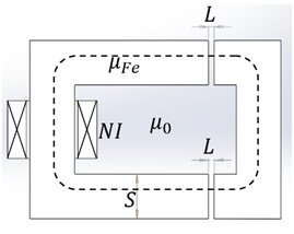
A magnetic circuit refers to a physical system comprised of components designed to generate and confine magnetic flux. Typically, this flux is generated by either permanent magnets or coils, with the flux paths being constructed from high-permeability ferromagnetic materials, such as iron. In Figure 1, we observe an illustration of a magnetic circuit [1] that includes two iron components with a specific cross-sectional area$$ S = 4 \, \text{cm} $$.
One part is stationary and the other is moving; they are separated by two air gaps of length -turn coil wrapped around the stationary part, carries the current I ( ) and is responsible for the flux in the circuit.
Force on the moving part can be determined by calculating the change in the magnetic energy $$ W \rightarrow W + 1 $$ that would be produced by moving the part over a small distance $$ L \rightarrow L + 1 $$. Force magnitude is obtained as:
F = \frac{\Delta W}{\Delta L}
$$
(eq.1)
This simple method is based upon the virtual displacement principle and it is often used to calculate forces in magnetic devices.
Since the permeability of iron is much greater than the permeability of air ($$
\mu_{\text{Fe}} \gg \mu_0
$$
), the magnetic field in the iron ($$
H_{\text{Fe}} = \frac{B}{\mu_{\text{Fe}}}
$$
), as well as leakage flux, are neglected. Ampere’s law for the contour in Figure 1. can be written as:
2 L H_a = N I
$$
(eq.2)
where represents the magnetic field in the air gap.
With no leakage and no field in the iron ($$
H_{\text{Fe}} \approx 0
$$
), the entire magnetic energy of the system is stored in the volume of the air gap and can be computed as:
W = \frac{1}{2} \int_V B H_a \, dV = \frac{1}{2} \int_V \mu_0 H_a^2 \, dV
$$
(eq. 3)
Assuming uniform field distribution in the air gap allows to calculate by simply multiplying energy density $$
\frac{1}{2} \mu_0 H_a^2
$$
and volume . The circuit contains 2 air gaps, therefore, after doubling the energy in eq.3 and substituting eq.2 in eq.3:
$$
W = \frac{1}{4} \mu_0 S \frac{(N I)^2}{L}
$$
(eq. 4)
For two different air gap lengths and , the change in magnetic energy can be computed as:
$$
\Delta W = W_2 - W_1 = \frac{1}{4} \mu_0 S (N I)^2 \frac{L_1 - L_2}{L_1 L_2}
$$
(eq. 5)
Equation 5, combined with eq. 1, yields the following expression for force magnitude:
$$
F = \frac{1}{4} \mu_0 S \frac{(N I)^2}{L_1 L_2} = 3.02 \, \text{N}
$$
(eq. 6)
MODEL
To accurately represent the situation in the analytical example, where force has been computed using energies for and air gaps, the CAD model of the circuit has been created with two air gaps of different lengths: and (Figure 2.).
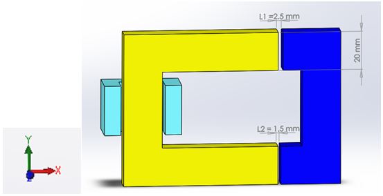
To exploit the problem's inherent symmetry, it suffices to simulate just one-half of the space, corresponding to half of the magnetic circuit. The simulation is conducted using the EMS Magnetostatic study, with a symmetry factor set at 0.5.
Current current-driven Wound Coil with turns and is added to the coil region. Its Entry and Exit Ports are faces in the plane of symmetry.
Material
The following instructions outline the process for creating a new material library, defining a custom material, and applying that material to an element within your model:
- In the EMS Manager tree, right-click the Stationary element icon in the Materials folder and select Apply Material to All Bodies. The Material Task Pane opens.
- Select “New Library
 from the “Material Task Pane”.
 - Browse to the location where to save the new library file (the file extension will be .emsmtr).
- Type MyLib for the name. An empty material library with the MyLib is added to the Material Task Panel.
- Click on Add Materiel button
 .
. - Type Mur1200 for the material's name.
- Click OK
 .
. - Type 1200 for the Relative Permeability and take the default for the rest of the fields.
- Click OK
 .
.
Copper is assigned to the coil region, and air to the surrounding volume.
Boundary Conditions
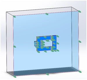
Figure 3 - Tangential Flux boundary condition
The normal component of the flux density at the plane of symmetry ( plane in Figure 2.) is zero (all flux lines are parallel to this plane). Therefore, the Tangential Flux boundary condition should be applied on all surfaces that belong to the plane, including air and coil cross-sections. To do so:
- In the study, right-click the Load/Restraint
 folder and select Tangential Flux. The Tangential Flux Property page appears.
 - Click inside the Faces for Tangential Flux box
 then select all the symmetry faces.
 - Click OK
 .
.
Coils
To add a coil to a Magnetostatic study:
- In the EMS manger tree right-click on the Coils
 icon and select Wound Coil
 .
. - Keep default Coil Type as a Current driven coil.
- Click inside the Components or Bodies for Coils box
 .
. - Click on the (+) sign in the upper left corner of the graphics area to open the components tree.
- Click on the Coil-1 icon. It will appear in the Components and Solid Bodies list.
- Click inside the Faces for Entry Port box
 then select the entry port face.
 - Click inside the Faces for Exit Port box
 then select the exit port face.
General Properties:
- Click on General properties tab.
- Type 300 in the Turns box
 .
. - Keep the default value of 1 the Current per Turn field
 . The units in Amp-Turns.
 - Click OK
 .
.
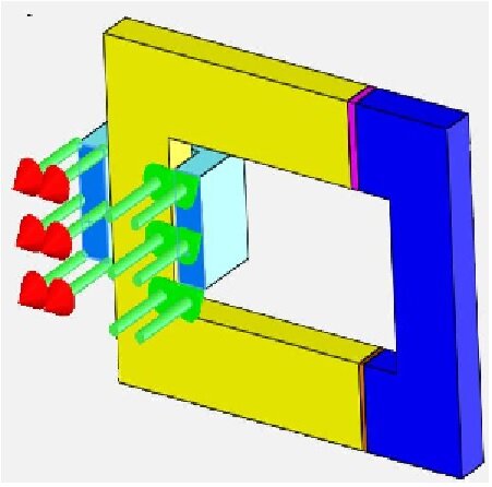
Figure 4 - Entry and exit ports of the coil
Force
EMS automatically calculates the distribution of nodal forces without requiring any user input. However, when it comes to calculating forces or torques on a rigid body, it is necessary to define the specific part on which the force or torque should be computed before initiating the simulation.
- In the EMS manager tree, right-click the Force/Torques
 folder and select Virtual Work
  .
. - The Forces/Torques Property Manager appears.
- Click inside the Components and Bodies for Forces/Torques box
 .
. - Click on the (+) sign in the upper left corner of the graphics area to open the components tree.
- Click on Moveable part icon. It will appear in the Components and Solid Bodies list.
- Click OK
 .
.
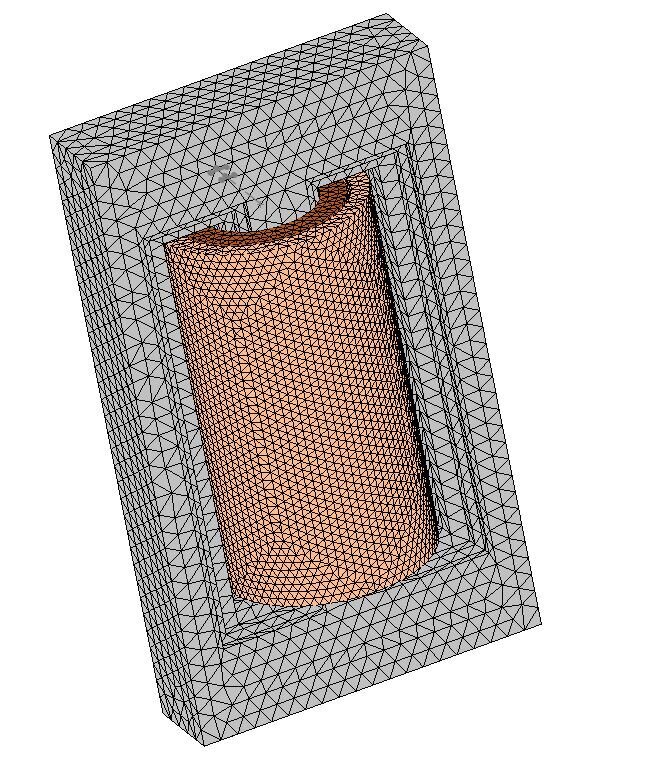
Mesh
The quality of the mesh in the air gap region is of critical importance for accurate force calculation. EMS allows user to take full control over the mesh resolution.
- In the EMS manager tree, right-click the Mesh
 icon and select Apply Control
  . The Mesh Control Property Manager Page appears.
 - Click inside the Components and Solid Bodies box
 .
. - Click on the (+) sign in the upper left corner of the graphical area to open the components tree.
- Click on the Air Gap 1, and Air Gap 2 icons. They will appear in the Components and Solid Bodies list.
- Under Control Parameters click inside the Element Size
 box and type 2.5 mm.
 - Click OK
 .
.
To mesh the model:
- In the EMS manager tree, right-click on the Mesh
 icon and select Create Mesh
  .
. - Type 35 in the box for an average number of mesh elements per diagonal for each solid body
 .
. - Click OK
 .
.
Right-click Study icon and select Run ![]() , to execute the simulation. Once the computation is done, the program creates five folders in the EMS manager tree. These folders are Report, Magnetic Flux Density, Magnetic Field Intensity, Current Density, and Force Distribution.
, to execute the simulation. Once the computation is done, the program creates five folders in the EMS manager tree. These folders are Report, Magnetic Flux Density, Magnetic Field Intensity, Current Density, and Force Distribution.
RESULTS
Flux density
It is a good habit to first view the magnetic flux density in the model, including the outer air. This action indicates whether the outer air boundary is far enough.
- In the EMS Manager tree, right-click on the Magnetic Flux Density folder and select 3D Fringe Plot> No Clipping.The Magnetic Flux Density Property Manager Page appears.
- In the Display box:
a. Select Br from the magnetic flux density component ![]() . Directions are based on the global coordinate system.
. Directions are based on the global coordinate system.
b. Set Units ![]() to Tesla.
to Tesla.
c. Select Continuous from Fringe Options ![]() .
.
3. Select OK ![]() .
.
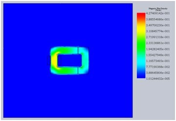
By examining Figure 5. it becomes clear that the magnetic flux density is very small on the outer air boundary. Thus, the air box is large enough. Had it been otherwise, the air box surrounding the magnetic circuit would have to be larger.
Force
In the EMS Manager tree, Double-click Result Table to display the force result.
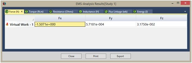
Remember that, because of the symmetry about the xy plane, only half of the problem has been modeled. Thus, and components must be multiplied by a factor of 2, while the component cancels out. Since is very small compared to , the resultant force is virtually in the X direction with a magnitude of . The analytical solution compares very well with the EMS result.
| Analytical Virtual Work Solution | EMS Result | |
| Force [N] | 3.02 | 3.014 |
Conclusion
The application note delves into the physics and simulation of magnetic circuits, focusing on force computation within a specific configuration. Through analytical derivations and simulation in Solidworks EMS Magnetostatic study, the note demonstrates the calculation of forces using principles like Ampere's law and virtual displacement. Key components such as iron cores, air gaps, and coils are meticulously modeled, with materials assigned and boundary conditions set accordingly. The simulation results, including magnetic flux density and force distribution, are compared with analytical solutions, showcasing close agreement and validating the simulation approach. By accurately capturing the behavior of magnetic circuits, the note offers valuable insights for engineers working in electromagnetics and device design. Additionally, it provides practical guidance on modeling techniques and simulation setup.
References
[1] Electromagnetics and calculation of fields, by Nathan Ida and Joao P. A. Bastos, 2nd Edition, page 183-184. Publisher: Springer-Verlag;