TEAM 24
TEASM 24 serves as a benchmark for 3D time-transient electromagnetic simulations. A test rig, resembling a Switched Reluctance Machine, consists of solid medium-carbon steel and is enclosed within a non-magnetic cage. The cage rotates around a stainless-steel shaft. Refer to Figure 1 for the dimensions of the test rig, with both the stator and rotor possessing a thickness of 25.4 mm. The geometric parameters of each pole coil are illustrated in Figure 2. Notably, the rotor is inclined at an angle of 22 degrees [1]. Additionally, Figure 3 depicts a detailed 3D model of the simulated test rig, providing a comprehensive view for analysis and interpretation.
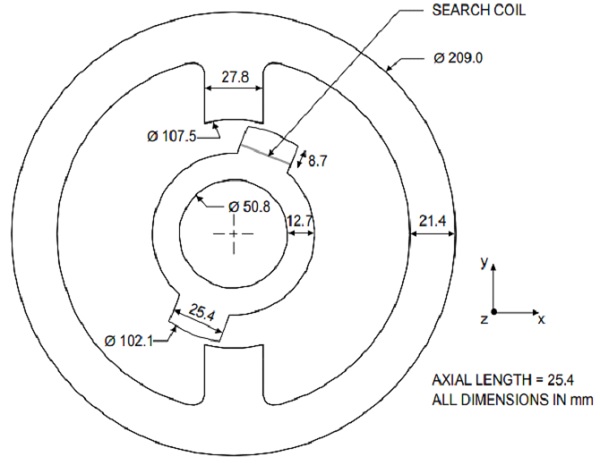
Figure 1 - Dimensions of stator and rotor.
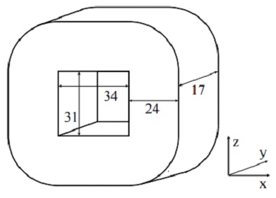
Figure 2 - Dimensions of the coils.
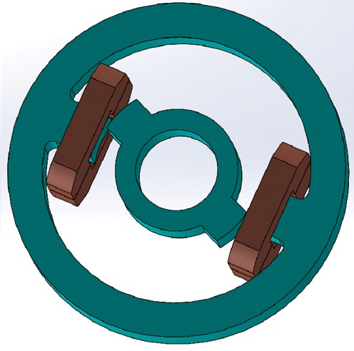
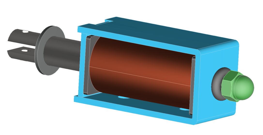
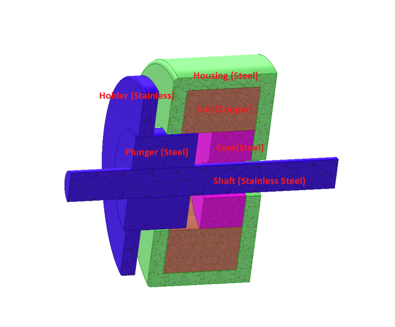
Figure 3 - CAD model of the test rig.
Time domain Simulation
To conduct a transient magnetic analysis using the EMS module, follow these simplified steps:
1. Create a Transient Magnetic Study: Initiate a new study in EMS, choosing "Transient Magnetic" as the study type to analyze time-varying magnetic fields.
2. Assign Materials: Select appropriate materials for all parts of your model. Each material's magnetic properties, like permeability, should match the real-world materials you're simulating.
3. Apply Coil Excitation: Decide whether your coil will be voltage-driven or current-driven and set the correct excitation. This involves specifying how the coil's excitation changes over time, whether through direct current, voltage levels, or a defined waveform.
4. Run the Simulation and Analyze Results: Execute the simulation to compute magnetic fields, eddy currents, and other relevant parameters over time. Use EMS's visualization tools to examine these results and gain insights into your design's electromagnetic performance.
This process allows you to model and understand the behavior of electromagnetic systems with time-varying fields, crucial for optimizing designs and improving performance.
Materials
After initiating a transient magnetic study, proceed to material assignment for each component:
- Stator and Rotor: Utilize EN9 steel, notable for its electrical conductivity of 4.54e+6 S/m and the BH curve depicted in Figure 4.
- Coils: Choose copper, recognized for its high electrical conductivity of 57.7e+6 S/m.
- Other Parts: Apply air to the remainder, accounting for the non-conductive and non-magnetic space surrounding the components.
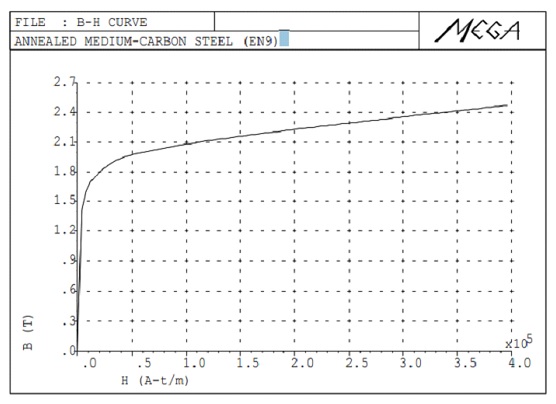
Figure 4: Measured initial magnetization curve[1] .
Coil excitation
For your transient magnetic study, define the coil with 350 copper turns, leveraging copper's conductivity of 57.7e+6 S/m, and apply the input current characteristics as depicted in Figure 5. Adjust the simulation to accurately reflect these dynamics, enabling a focused analysis on how the input current influences magnetic field variations and overall performance, ensuring a precise understanding of the winding's electromagnetic behavior.
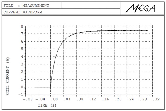
Figure 5 - Input current for each winding.
To compute the magnetic force and torque produced on the rotor, a virtual work on the rotor is defined.
Mesh
Mesh quality is crucial for the accuracy and efficiency of FEM simulations. EMS's Mesh Control feature allows users to finely adjust mesh sizes on solid bodies and faces, optimizing computational resources and result precision. This balance is key in areas of varying complexity, enhancing detailed analysis while managing solving time. The applied mesh controls, detailed in Table 1 and visualized in Figure 6, demonstrate the strategic distribution of mesh density across the model to achieve optimal simulation outcomes.
Table 1: Applied mesh controls
| Bodies / components | Mesh control size |
| Coils and shaft | 6 mm |
| Stator and rotor | 4 mm |
| Air gaps | 0.5 mm |
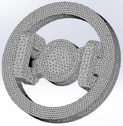
Figure 6 - Meshed model.
Results
Upon completing the simulation, EMS generates a comprehensive set of results crucial for analyzing the electromagnetic behavior of the model. These results include:
-
Magnetic Flux Density: The distribution of magnetic flux across the model.
-
Magnetic Field Intensity: The strength of the magnetic field at various points.
-
Eddy Current: Currents induced by changing magnetic fields, affect both stator and rotor.
-
Inductance & Impedance: Key parameters influencing the circuit's reactive properties.
-
Flux Linkage: The interaction between the magnetic field and the coil windings.
-
Current & Induced Voltage: The electrical response of the system to electromagnetic phenomena.
-
Force & Torque: Mechanical outputs from electromagnetic interactions, critical for motion analysis.
-
Losses: Energy dissipated in various forms, impacting efficiency.
Figures 7 and 8 illustrate the magnetic flux density with fringe and vector plots, capturing its spatial distribution at two distinct moments (0.24 sec and 0.195 sec), offering insights into the dynamic magnetic behavior. Figure 9 focuses on the eddy currents induced in both the stator and the rotor, highlighting areas of potential energy loss or heating, which are critical for the design and optimization of electromagnetic systems. These visualizations not only aid in the interpretation of complex electromagnetic phenomena but also provide a basis for refining designs to enhance performance and efficiency.
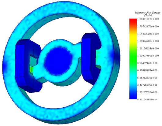
Figure 7 - Fringe plot of the magnetic flux density at 0.24 s.
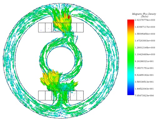
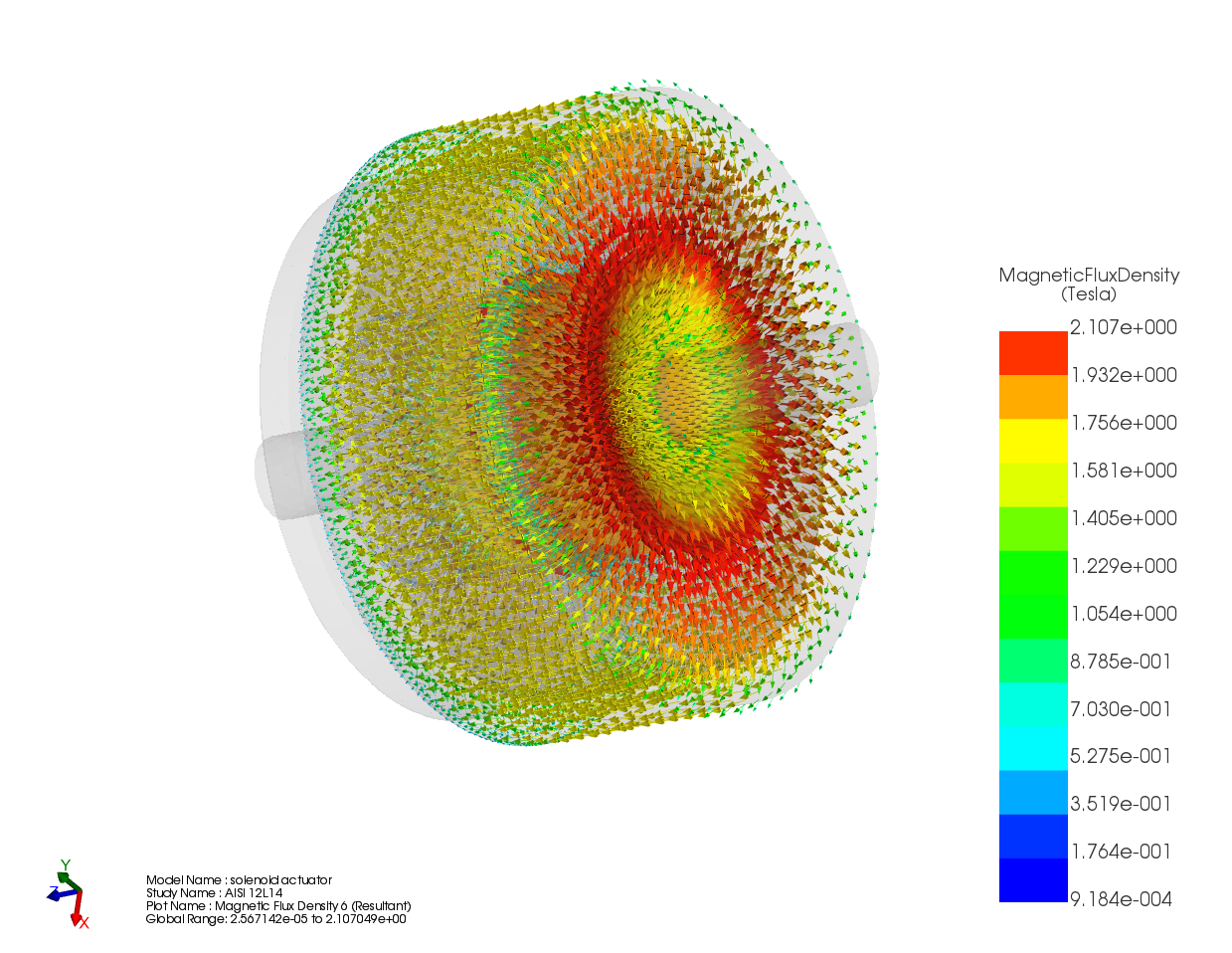
Figure 8 - Vector plot of the magnetic flux density at 0.195 sec on the middle section of the model.
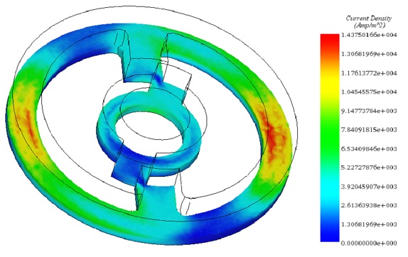
Figure 9 - Eddy current density at 0.17 sec.
Figure 10 presents a comparative analysis of torque variation results obtained from EMS simulations against those from the TEAM 24 benchmark. This comparison is crucial for validating the accuracy and reliability of EMS simulations in predicting electromagnetic behavior. The plot indicates that the torque variations predicted by EMS closely align with the benchmark results from TEAM 24, demonstrating good agreement.
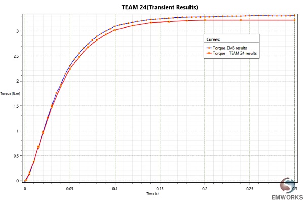
Figure 10 - Torque result comparison.
Conclusion
The application note on TEAM 24 explores the capabilities of 3D time-transient electromagnetic simulations through the case study of a Switched Reluctance Machine test rig. This detailed study utilizes the EMS module for transient magnetic analysis, focusing on material selection, coil excitation, and the execution of simulations to understand time-varying magnetic fields and their effects. Key components like the stator, rotor, and coils are carefully selected based on their electromagnetic properties to accurately model and simulate the electromagnetic behavior of the system.
The simulation process outlined, from initiating a transient magnetic study to meshing and analyzing results, enables a comprehensive understanding of the electromagnetic system's performance. The study meticulously applies appropriate materials and excitation inputs to model the system, culminating in an analysis that includes magnetic flux density, field intensity, eddy currents, and mechanical outputs such as force and torque. The findings, illustrated through various figures, offer insights into the electromagnetic phenomena within the machine, highlighting areas of potential optimization.
Notably, the comparison of EMS simulation results with the TEAM 24 benchmark validates the accuracy and reliability of the simulation, demonstrating the utility of EMS in predicting electromagnetic behavior. This application note underscores the significance of detailed electromagnetic simulations in designing and optimizing electromagnetic systems, providing a foundation for enhancing the efficiency and performance of devices like the Switched Reluctance Machine.
References
[1] http://www.compumag.org/jsite/images/stories/TEAM/problem24.pdf