TEAM 20
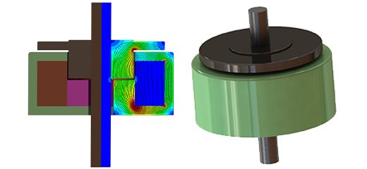
Analyze a solenoid example (TEAM 20) featuring a steel core and plunger pole, as illustrated in Figure 1, utilizing EMS's magnetostatic solver. The pole armature experiences a force generated by the current applied to the surrounding coil.
This scenario corresponds to TEAM Workshop problem #20, initially introduced by Nakata et al [1]. The initial findings and measured data can be found in [2], with additional measured results presented during the TEAM-Workshop [3]. The results section will include a comprehensive comparison with the measured data.
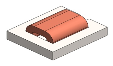
Figure 1 - Dc Solenoid
Study
In the solenoid depicted below in Figure 2, the central pole and yoke are constructed from steel, while the coil is composed of copper and energized by a DC current of 3000 A-turns, with N = 3000 turns and a current of 1 A per turn. This current level is ample to saturate the steel material. Consequently, this specific scenario necessitates a solution through nonlinear Magnetostatic analysis. Once more, to capitalize on the inherent symmetry, only half of the problem is modeled.
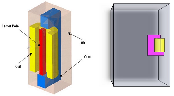
Figure 2 - 3D Model of the DC Solenoid
Materials
In the context of the Magnetostatic study, the essential property required is the relative permeability of each material.
Table 1 - Materials information
| Components / Bodies | Material | Relative permeability |
| Center_pole | MA2-Steel | Non linear |
| Coil | Copper | 0.99991 |
| Inner_air | Air | 1 |
| Outer_air | Air | 1 |
| Yoke_T | MA2-Steel | Non linear |
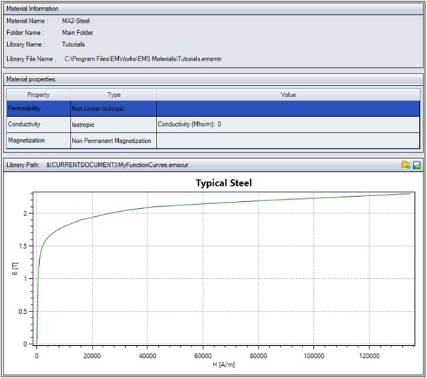
In this particular problem, MA2-Steel (Figure 3) is a non-linear material. The EMS Materials Library conveniently offers a dedicated folder for non-linear materials, allowing for the easy retrieval or addition of BH curves.
Loads and restraints
Loads and restraints play a crucial role in defining the electric and magnetic environment within the model. The accuracy and relevance of analysis results are directly influenced by the specific loads and restraints defined. These loads and restraints are applied to geometric entities as features, and they maintain full association with the geometry, automatically adapting to any geometric modifications or changes.
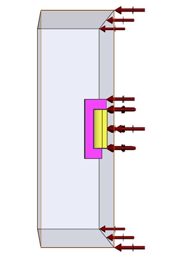
In this study, a coil (refer to Table 2) is applied as a component, and the Center of pole serves as a Load (refer to Table 3). The primary objective is to calculate the virtual work associated with these elements.
Table 2 - coil information
| Name | Number of turns | Magnitude |
| Wound Coil | 3000 | 1 A |
Table 3 - Force and Torque information
| Name | Torque Center | Components / Bodies |
| Virtual Work | At origin | Center_pole |
Meshing
To optimize meshing, the air region has been divided into two distinct parts: inner air and outer air. This approach is strongly recommended for most problems since it allows for a dense mesh in the inner air regions where the field is significant while utilizing a coarser mesh in the outer air regions where the field typically diminishes. This method effectively captures the field variation in the relevant areas without the need for an excessive number of mesh elements.
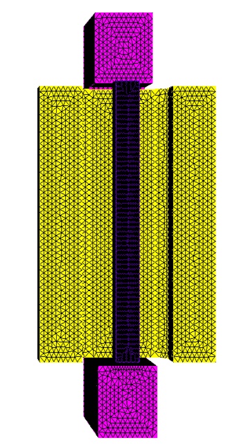
Mesh quality adjustments can be made using Mesh Control (see Table 4), which can be applied to solid bodies and faces. As illustrated in Figure 4 below, the model has been meshed using Mesh Controls, resulting in an optimized mesh configuration.
Table 4 - Mesh control
| Name | Mesh size | Components /Bodies |
| Mesh control 1 | 2.00 mm | Coil_T, /Yoke_T |
| Mesh control 2 | 0.5700 mm | Center_pole-1 |
Results
Following the simulation of this example, a variety of results can be obtained using the Magnetostatic Module. These results include:
-
Magnetic Flux Density (as shown in Figure 6).
-
Magnetic Field Intensity.
-
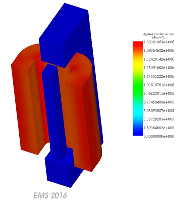
Applied Current Density (as depicted in Figure 7).
-
Force Density.
-
Field Operation, including derivatives of B and H.
-
A result table (refer to Figure 9) containing computed parameters of the model, force, and torque.
Additionally, EMS enables the generation of 2D plots, as illustrated in Figure 8. This wide range of results allows for a comprehensive analysis of the magnetic behavior in the modeled system.
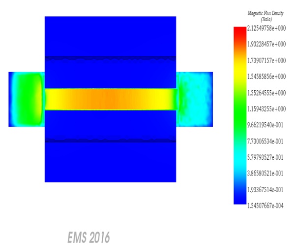
Figure 6 - Magnetostatic Flux density , fringe plot
Verifying the Flux density results
One of the benchmark results specified by TEAM 20 is the calculation of the average magnetic flux density along the Z-axis (Bz) at the midpoint of the center pole [1]. The corresponding measured data can be found in [3].
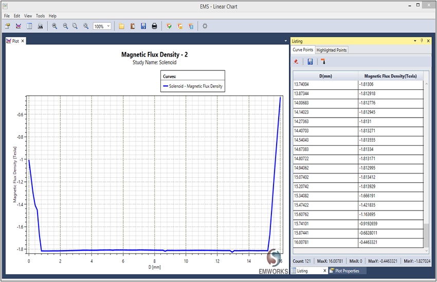
The measured data in [3] provides the average Bz value. To calculate the average value from the obtained results, you can save the data to an Excel file (.xls) and perform the necessary calculations. It appears that the calculated average Bz is approximately -1.71 T, which closely matches the -1.75 T value reported in [2]. This alignment suggests good agreement between the simulation results and the reported benchmark data.
Verifying the Force results
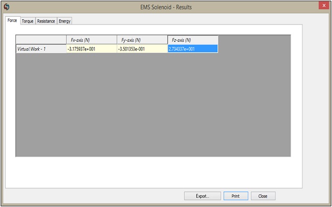
Indeed, due to the symmetry of the problem with the plane of symmetry orthogonal to the X-axis, certain force components are affected as follows:
-
The Fy and Fz components need to be multiplied by a factor of 2.
-
The Fx component cancels out due to the symmetry.
Given that Fy is considerably smaller than Fz, the resultant force is entirely in the Z direction and has a magnitude equal to 2 times the calculated value, which is 2 x 27.34 = 54.68 N.
When comparing this obtained force of 54.68 N to the measured force of 54.4 N [3], the results fall within an acceptable difference, indicating a good alignment between the simulation and the measured data.
Conclusion
The application note delves into the analysis of a solenoid example, TEAM 20, utilizing EMS's magnetostatic solver. This study examines the force experienced by the pole armature due to the current applied to the surrounding coil, focusing on a specific problem introduced by Nakata et al. The analysis involves material properties, loads, restraints, meshing strategies, and result interpretation. Meshing optimizations and result verification against benchmark data ensure accuracy and reliability. The simulation yields magnetic flux density, field intensity, force density, and more. Comparisons with measured data demonstrate the simulation's validity, affirming good alignment between calculated and experimental results. This comprehensive study enhances understanding of solenoid behavior and validates EMS's magnetostatic solver for similar applications.
References
[1] T. Nakata, N. Takahashi, and H. Morishige, "Proposal of a model for verification of software for 3-d static force calculation," in Verification of Software for 3-D Electromagnetic Field Analysis (Z. Cheng, K. Jiang, and N. Takahashi eds.), pp. 139-147, 1992.
[2] T. Nakata, N. Takahashi, H. Morishige, J. L. Coulomb, and J. C. Sabonnadiere, "Analysis of 3-d static force problem," in Proceedings of TEAM Workshop on Computation of Applied Electromagnetics in Materials, pp. 73-79, 1993.
[3] T. Nakata, N. Takahashi, M. Nakano, H. Morishige, and K. Masubara, "Improvement of measurement of 3-d static force problem (problem 20)," in Proceedings of TEAM Workshop , Miami, November 1993.