Magnetic Resonance Imaging (MRI)
Magnetic Resonance Imaging (MRI) is a medical imaging method employed in radiology to identify and address abnormal medical conditions. MRI machines utilize robust magnetic fields, radio waves, and field gradients to produce detailed images of the body's internal organs. It's important to note that MRI does not involve the use of X-rays. Generally, MRI is considered a safe technique, although injuries can occur if safety protocols are not followed diligently.
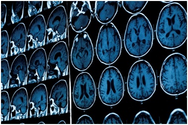
One notable advantage of MRI is that it doesn't expose patients to ionizing radiation, making it a preferred choice over CT scans when both methods can yield similar diagnostic results. However, there are situations where MRI may not be the preferred option due to factors such as cost, time consumption, and potential discomfort, especially for individuals who experience claustrophobia. For reference, Figure 1 illustrates an MRI image.
Problem description
In this example, EMS serves two main purposes. Firstly, it is utilized to validate Finite Element Analysis (FEA) results by comparing them to theoretical formulas. Secondly, EMS is employed to simulate the MRI coil. To achieve these objectives, both the Magnetostatic and Transient solvers within EMS are utilized.
Validation of FEA results
Magnetic flux density validation using EMS
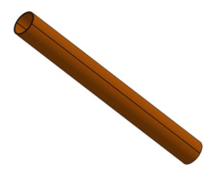
To validate the accuracy of the EMS software for modeling the magnetic field (B field), Ampere's Law is employed. In this validation process, a solenoid is intentionally designed with specific parameters, including 100 turns of #18 AWG copper wire, a diameter of 1.02362 mm, and a current supply of 1.0 A. Ampere's Law is then applied to analyze the magnetic field within the solenoid.
$$ B = \mu N I = \mu_0 \mu_r N I $$
Where $$ \mu $$ is the magnetic permeability of copper, $$ \mu_0 $$ is the permeability of free space, $$ \mu_r $$ is the relative permeability of copper, N is the number of turn and I is the current of coil.
Applying the formula mentioned above, the previous coil is expected to generate a magnetic flux of 1.23 e-3 T [2].
In Figure 2 below, you can observe the simulated reference coil. Due to the DC excitation used, performing a Magnetostatic study within EMS is essential to accurately simulate this coil.
Study
The Magnetostatic module within EMS is employed to calculate and visually represent various magnetic parameters within the coil. This includes magnetic flux, magnetic intensity, current density, and inductance of the coil. When setting up a Magnetostatic study in EMS, it is crucial to adhere to the following four essential steps:
- apply the proper materials for all solid bodies.
- apply the necessary boundary conditionsor Loads/Restraints in EMS.
- mesh the entire model.
- run the solver.
Materials
The coil is made of copper. Below are the properties of copper in the magnetostatic study.
| Relative permeability | Electrical conductivity S/m | |
| Copper | 0.99998 | 58.00e+6 |
| Air | 1 | 0 |
Loads and restraints
To define our study, a coil must be added. In Table 2, the coil properties are listed.
| Number of turns | Current magnitude | |
| Solid Coil | 1 | 1 A |
A virtual work approach is employed within the square loop to calculate the torque applied to it. This method allows for the determination of the torque experienced by the loop in response to external forces or conditions.
Meshing
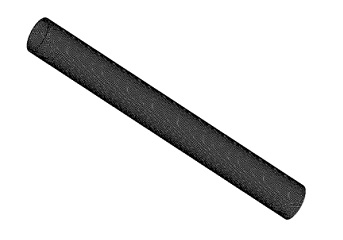
In design analysis, EMS optimizes meshing by considering the model's specifics, and adjusting element size for accuracy or speed. Early stages might use larger elements for quick, rough results, while detailed studies require finer meshing. EMS's Mesh Control enhances precision in critical areas, as depicted in Figure 3, where a 0.5 mm control refines the coil's mesh for targeted analysis..
Results
Following the completion of the simulation in the magnetostatic study, a range of valuable results can be obtained, including:
- Magnetic Flux Density: This parameter quantifies the distribution of magnetic flux within the analyzed system.
- Magnetic Field Intensity: It represents the strength and direction of the magnetic field.
- Applied Current Density: This parameter characterizes the current density distribution within the coil.
- Force Density: It describes the distribution of forces acting on the analyzed components.
Additionally, a results table is provided, containing circuit parameters and various magnetic quantities. Figure 4 visually displays the magnetic flux distribution within the reference coil, with both theoretical and EMS simulation results matching closely. A 2D plot (Figure 5) further illustrates that the magnetic flux exhibits a nearly uniform distribution along the axis of the coil. This congruence between theoretical and simulation results validates the accuracy of the analysis conducted using EMS.
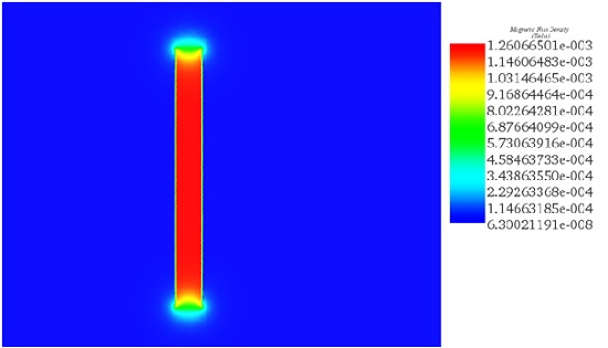
Figure 4 - Magnetic flux in reference coil
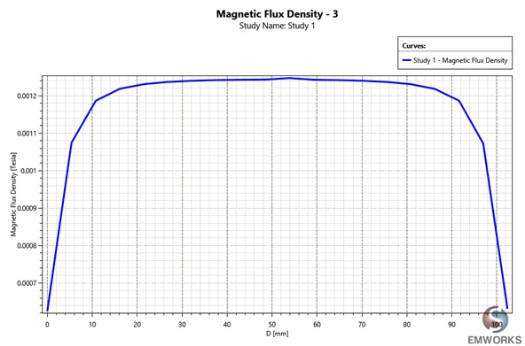
Figure 5 - Magnetic flux a long the coil axis.
Torque validation using EMS
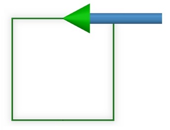
In addition to verifying EMS's capability to generate the magnetic field (B field), it is essential to validate the accuracy of torque calculations. For this validation, a commonly used configuration involving a square loop is employed. The square loop utilized in this simulation has a 1 mm square cross-section and is situated within a 100 mm x 100 mm square loop, positioned at the center of the magnetic field bore.
The square loop conducts a DC current of 1 A and is immersed in a uniform magnetic flux of 1.56 T. To generate this magnetic flux using Ampere's Law for a solenoid, a random coil configuration is created. Figure 6 illustrates the square loop with the initial current direction positioned in the XZ plane. Subsequently, the loop is incrementally rotated in the x-axis, ultimately reaching a 90-degree rotation where the loop lies in the XY plane [2]. This setup allows for the verification of torque calculations in different orientations of the square loop.
In our case the torque is calculated by the formula below:
$$ B = LAB \cdot \sin(\theta) $$
$$ \theta $$ is the angle between the B field vector and the magnetic moment vector. The magnetic moment of a current loop is simply IA, where I is the current in the loop and A is the area of the loop immersed in the B field.
Study
In this simulation, we will follow the same steps as in the previous section to analyze and validate the torque calculations for the square loop configuration.
Materials
The current square loop is constructed from copper material. Here are the essential copper properties required for the magnetostatic study without any coupling:
Table 1 - Copper properties
| Relative permeability | Electrical conductivity S/m | |
| Copper | 0.99998 | 58.00e+6 |
| Air | 1 | 0 |
Loads and restraints
To define our study, a solid coil must be added. In table 2, the coil properties are listed.
Table 2 - Coil properties
| Number of turns | Current magnitude | |
| Solid Coil | 1 | 1 A |
A virtual work approach is applied within the square loop to calculate the torque. This method allows for the determination of the torque experienced by the loop based on virtual work principles.
Meshing
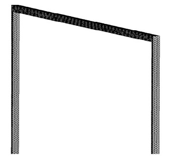
Figure 6 displays a section of the meshed model, specifically focusing on the square loop. Mesh control with a size of 0.3 mm has been applied to ensure a finer level of detail in the mesh within this region of the simulation.
Results
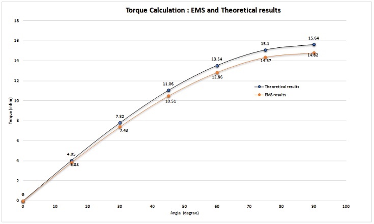
Here is a comparison between the torque results obtained from EMS simulations and theoretical calculations at various angles. This comparison serves to validate the accuracy of EMS's torque calculations in different orientations of the square loop.
3D simulation of Bore coil used in MRI
The bore coil, also known as the MRI bore magnet, is a crucial component used to generate a high and uniform magnetic flux within the MRI machine. This bore magnet is designed in the form of a relatively long solenoid to achieve the goal of creating a uniform magnetic field. In typical MRI machines, the dimensions of the bore are approximately 36 inches in diameter and can range from 36 to 72 inches in length.
For the purpose of this design, we have adopted a more convenient measurement system, with a bore diameter of 100 cm and a length of 200 cm. To ensure that the bore magnet solenoid has sufficient mass for the stranded currents, the outer radius of the bore magnet is set at 200 cm [2]. Figure 9 illustrates the MRI bore magnet, which has been modeled using SolidWorks.
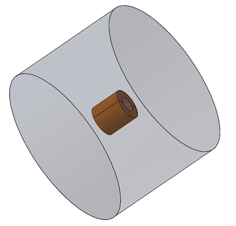
Figure 9 - 3D model of bore coil with air surrounding
In this simulation, the Magnetostatic solver in EMS for SolidWorks was utilized. A wound coil, specifically a single-turn coil excited by a DC current of 2983900, was applied as the load. To enhance visualization of the magnetic flux within the coil, an inner air space was included in the model. Prior to running the simulation, mesh control was applied to the inner air to ensure accurate results. The simulation setup mirrors the one used for the reference coil simulation in section 1.
Figure 10 provides a visualization of the magnetic flux generated by the bore coil, demonstrating that the magnetic field (B) is nearly uniform within the coil. Figure 11 focuses on the magnetic flux plotted exclusively in the inner air (inside the coil), revealing that the flux is aligned along the z-axis.
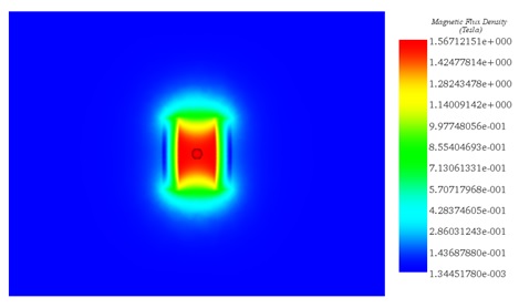
Figure 10 - Magnetic flux density created by a bore coil
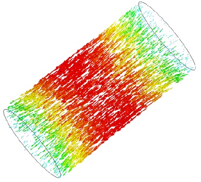
Figure 11 - Magnetic flux density, vector plot
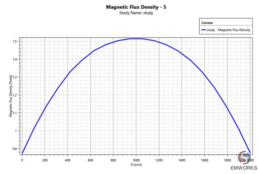
Figure 12 - 2D plot of the magnetic flux a long the z -axis
Simulation of MRI design
The simulated MRI system integrates a bore with gradient coils, each placed 1 mm from the bore and concentric, forming a complete system shown in Figure 13. This setup, reflecting a typical MRI's structure, includes three gradient coil sets, with the axial ones designed as solenoid or "Helmholtz" coils at the bore's ends. These coils are arranged to either augment or counter the bore coil's magnetic field, based on their current flow direction, utilizing AC current at 100 Hz for excitation. The use of both DC and AC currents necessitated the Transient solver in EMS for a dynamic simulation across two time frames (2/100 s). Figure 14 shows the magnetic flux along the z-axis at the sinusoidal current's peak, indicating the bore's axial field shape remains consistent despite the gradient coil's presence.
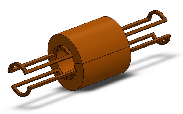
Figure 13 - 3D CAD model of MRI with bore and gradient coils.
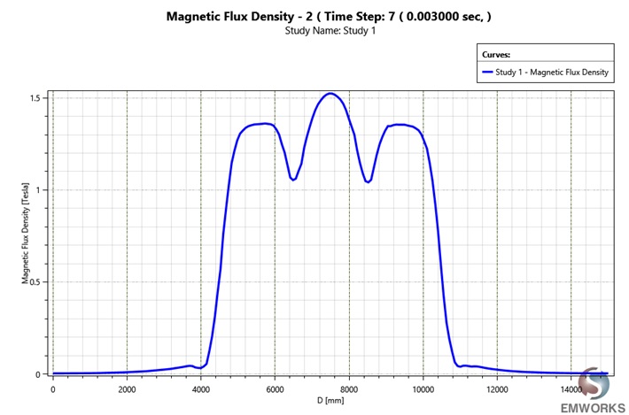
Figure 14 - Magnetic flux density along the z-axis at 0.003 second
Conclusion
This application note thoroughly investigates the design and simulation of an MRI system using EMS software, focusing on the accuracy of Finite Element Analysis (FEA) results and the simulation of MRI coils, including both Magnetostatic and Transient solver applications. Initially, the note validates the EMS software's capability to model magnetic fields using a reference solenoid coil, applying Ampere's Law for theoretical comparison and demonstrating a close match between simulation and theoretical predictions of magnetic flux density.
The exploration extends to validating torque calculations using a square loop in a magnetic field, showcasing EMS's precision in different orientations. The main study then transitions to the 3D simulation of an MRI bore coil, a critical component for generating a uniform magnetic field essential for MRI functionality. This bore magnet is simulated to assess the magnetic flux distribution, ensuring a nearly uniform field within the MRI.
Furthermore, the note delves into the simulated MRI system's construction, combining the bore and gradient coils to examine the influence of gradient coils on the axial magnetic field. Despite the introduction of gradient coils excited by AC current, the overall shape of the axial field inside the bore remains unaffected, underscoring the system's design efficiency.
In conclusion, the EMS simulations affirm their reliability for optimizing MRI coil designs and evaluating the magnetic flux's behavior, establishing EMS as a potent tool for MRI system study and enhancement. This validation of EMS's capabilities in both magnetic flux and torque calculations emphasizes its utility in advancing MRI technology.
References
[1]: https://en.wikipedia.org/wiki/Magnetic_resonance_imaging
[2]: RUSSELL L. CASE JR.2007: REDUCING EDDY CURRENTS IN HIGH MAGNETIC FIELD ENVIRONMENTS. University of Central Florida