TEAM problem 15
Non-destructive testing (NDT), crucial in sectors like aerospace and manufacturing for ensuring safety and quality, benefits significantly from eddy current testing (ECT). ECT, leveraging electromagnetism, excels in inspecting electrically conductive materials' surfaces without needing direct contact or coupling liquids. Its ability to detect surface flaws, subsurface irregularities, and material properties, including corrosion, highlights its versatility. Additionally, the integration of computer-aided design with ECT enhances its application, as seen in the validation of EMS results with TEAM problem 15, focusing on a rectangular slot in a thick plate.
Description and objective of the problem[1]
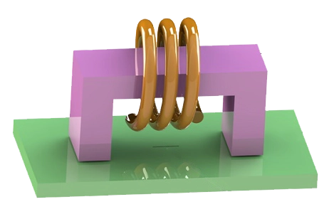
Figure 1 illustrates the experimental setup where a circular air-cored coil moves parallel to the x-axis over a slot in an aluminum alloy plate. During the test, the coil's frequency and lift-off distance are fixed, while changes in coil impedance, based on the coil's location, are precisely monitored. Key test parameters are detailed in Table 1.
This study aims to evaluate how coil impedance varies over different sections of the plate, comparing EMS results with benchmark data to validate the accuracy of the simulation.
Table 1- Parameters of simulation and test experiment
|
|
|
| Inner radius (mm) | 6.15 |
| Outer radius (mm) | 12.4 |
| Length (mm) | 6.15 |
| Lift-off (mm) | 0.88 |
|
|
|
| Thickness (mm) | 12.22 |
|
|
|
| Length (mm) | 12.60 |
| Depth (mm) | 5.00 |
| Width (mm) | 0.28 |
|
|
|
| Excitation frequency | 900 Hz |
| Skin depth | 3.04 mm |
| Isolated coil inductance | 221.8 mH |
Figure below shows a 3D CAD model of the simulated problem.
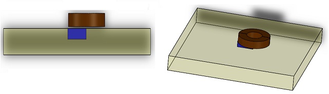
Figure 1 - CAD model of simulated NDT example
Exploring the AC Magnetic Module
The AC Magnetic module in EMS is instrumental for analyzing outcomes under sinusoidal excitation, including magnetic flux density, eddy current density, and loss density. It also sheds light on total eddy current loss, Joule loss, and the impedance matrix.
For an AC Magnetic simulation in EMS, these steps are crucial:
1. Initiate an AC Magnetic Study: Start by creating a new study focused on AC magnetic analysis.
2. Select Appropriate Materials: Assign the correct materials to each part based on their magnetic properties.
3. Define Coil Excitation: Choose between voltage or current-driven excitation for your coil and set the appropriate parameters.
4. Mesh and Execute the Simulation: With a focus on precision, utilize a finer mesh, especially in a half-model simulation to enhance accuracy and reduce computation time.
Materials
The coil in the simulation is crafted from copper, featuring a high conductivity rate of \(57 \times 10^7\) S/m, ensuring efficient electrical flow. The specimen material, on the other hand, has a conductivity of \(3.06 \times 10^7\) S/m, differentiating it from the coil in terms of electrical conductance.
Load Restraint
The sensor in this setup is the coil, with its properties meticulously detailed in Table 2.
Table 2 - Coil properties
| Number of turns | Current magnitude | Current frequency | |
| Wound Coil | 3790 | 6.15 A | 900 Hz |
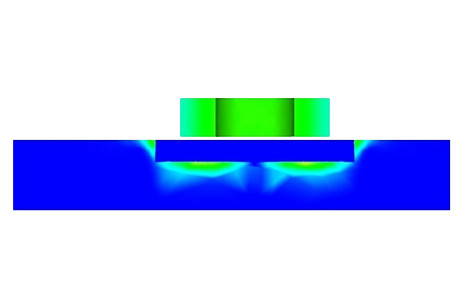
In this example, leveraging symmetry requires the addition of tangential flux on faces adjacent to the symmetry plane, as depicted in the accompanying figure.
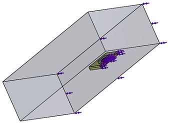
Figure 2 - Preview showing the applied tangential flux
Mesh
Mesh quality significantly influences the accuracy and computational efficiency of Finite Element Method (FEM) simulations. EMS enables detailed control over mesh sizes for various elements, enhancing simulation precision through its Mesh Control feature. In this case, the air domain surrounding the coil and the air within the crack are finely meshed, with the crack's mesh not exceeding a 0.1mm element size. To effectively manage the specimen's thickness, it is divided into two sections, allowing for specialized mesh control on the upper portion, as shown in Figure 3.
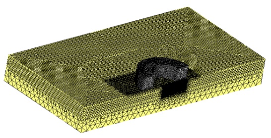
Figure 3 - Meshed Model
EMS results
EMS's parametric analysis feature allows for the sweeping of various parameters, including those related to geometry or simulation settings. In this study, the variable is the distance between the coil center and the crack, facilitating simulations for both flawed and flawless specimens. EMS uniquely compiles results from each scenario into one study, offering an integrated overview.
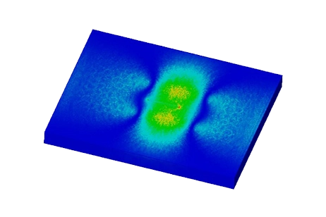
The computed inductance of the isolated coil by EMS stands at 214.98 mH. Figures 4 and 5 illustrate the comparison in eddy current distribution on the plate with and without the defect.
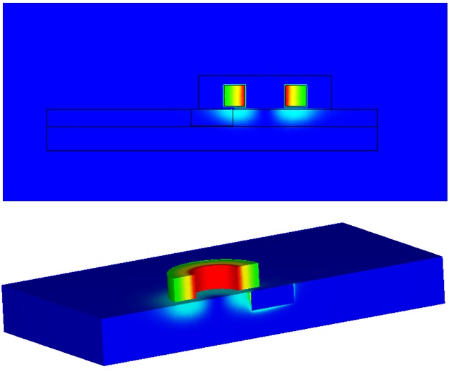
Figure 4 - Current density distribution in case of plate with a flaw
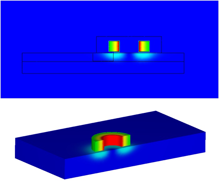
Figure 6 - Current density distribution in case of plate without a flaw
The absolute impedance is calculated as in the formula below:
Where X and R respectively the reactance and the resistance of the coil.
Figures 6 to 9 present a comparison between EMS outcomes and benchmark results for impedance and phase variation. The EMS solution shows excellent agreement with the TEAM 15 results, demonstrating its accuracy in simulating electromagnetic phenomena.
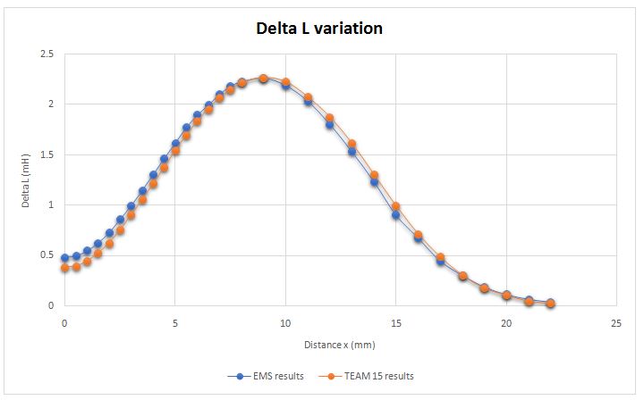
Figure 6 - EMS and benchmark results of delta L variation.
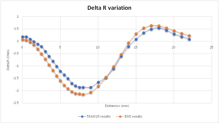
Figure 7 - EMS and benchmark results of delta R variation.
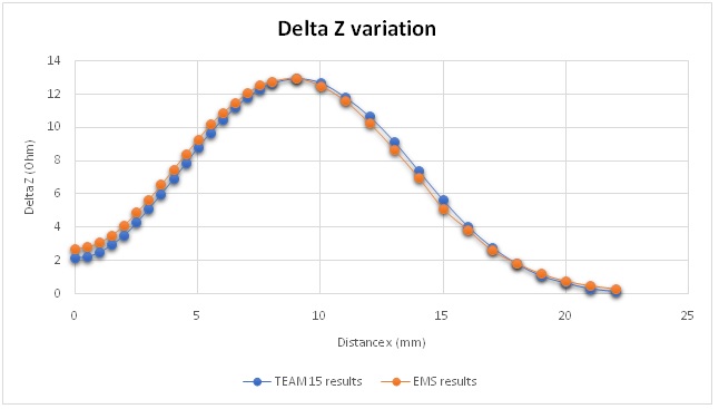
Figure 8 - Absolute impedance variation
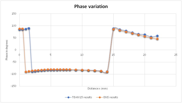
Figure 9 - Phase variation
Enhancing Eddy's Current Testing with EMS
The AC Magnetic module in EMS is crucial for accurately modeling eddy current effects on coil inductance and material losses, establishing EMS as the go-to tool for various Eddy current testing applications. This capability facilitates the creation of flaw detectors with enhanced efficiency, accuracy, and reliability for surface and subsurface inspections. The credibility of EMS's results is further confirmed by a detailed comparison with TEAM problem 15 outcomes, solidifying its status as a dependable and precise simulation solution.
Conclusion
This application note explores the utilization of EMS in the realm of non-destructive testing (NDT), specifically focusing on eddy current testing (ECT) for detecting defects in electrically conductive materials. ECT's ability to inspect without direct contact, leveraging electromagnetism, is highlighted through the analysis of TEAM problem 15, which examines a circular air-cored coil's impedance changes over a slot in an aluminum alloy plate.
EMS's AC Magnetic module is instrumental in simulating the eddy current effects, providing insights into magnetic flux density, eddy current density, loss density, and impedance variations. By comparing EMS results with benchmark data, the study validates the precision and reliability of EMS in simulating electromagnetic phenomena, particularly in identifying surface and subsurface flaws.
Key steps in conducting an AC Magnetic simulation include creating a new study, selecting appropriate materials, defining coil excitation, and executing the simulation with a focus on precision meshing. The study demonstrates EMS's powerful parametric analysis capability, allowing for the examination of flawed and unflawed specimens and the comparison of inductance values and eddy current distribution.
In conclusion, EMS emerges as a preferred tool for ECT applications, enhancing the efficiency, accuracy, and reliability of flaw detectors. The validation against TEAM problem 15 underscores EMS's credibility as a precise and dependable simulation tool in advancing NDT methodologies.
References
[1]: http://www.compumag.org/jsite/images/stories/TEAM/problem15.pdf