TEAM Benchmark 7
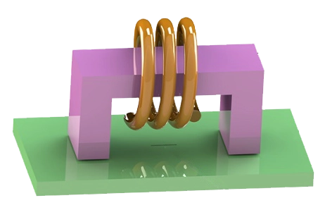
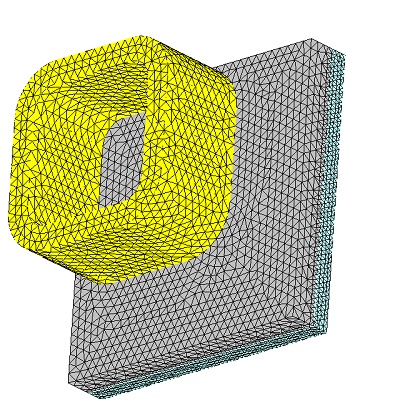
The TEAM Benchmarks initiated at Argonne National Laboratory in 1985, aim to showcase the efficacy of numerical techniques in solving electromagnetic field problems. The model depicted below features a thick aluminum plate with an eccentric hole and an exciting coil, modeled entirely due to its asymmetry. This problem is identified as TEAM Workshop problem #7, with detailed data and descriptions provided in [1]. Further measured results are available in [2], with a comparison to be presented in the results section.
Skin Depth Calculation
The initial stage for AC Magnetic problems involves computing the skin depth (d), representing the depth of penetration of the field into conducting regions. In this scenario, the skin depth in the Aluminum plate is calculated at a frequency of f = 50 Hz, using the formula:
We obtain d = 11.98 mm. The height of the Aluminum plate H = 19mm. Thus H/d = 19/11.98 = 1.58. Hence the current problem indeed requires the AC Magnetic analysis. Furthermore, as mentioned earlier, for the AC magnetic analysis, the mesh must have at least two elements per skin depth in the conducting regions where an eddy current is expected to be induced. Given a ratio of H/d = 1.58, 3 to 4 mesh elements along the height of the Aluminum plate are sufficient.
Since the coil is stranded, it does not support eddy currents. Therefore, there is no need to calculate the skin depth in the coil.
Study
The AC Magnetic module of EMS is instrumental in computing and visualizing magnetic fields induced by current or voltage surges. This analysis, which can be linear or non-linear, encompasses eddy currents, power losses, and magnetic forces. Upon creating an AC Magnetic study and coupling it with thermal analysis in EMS, four crucial steps must be followed: 1 - apply appropriate materials to all solid bodies, 2 - define necessary boundary conditions (Loads/Restraints), 3 - mesh the entire model, and 4 - execute the solver.
Materials
In the AC Magnetic analysis of EMS, comprehensive material properties are required for accurate simulation. These properties are detailed in Table 1 and include parameters such as electrical conductivity, relative permeability, and thermal conductivity.
| Components / Bodies | Material | Relative permeability | Conductivity (S/m) |
| Half Coil 1 / Half Coil 2 | Copper | 0.999991 | 5.7e+007 |
| Outer Air / Airb | Air | 1 | 0 |
| Plate | Aluminum | 1 | 3.526e+007 |
| Hole | Hole | 1 | 1 |
ElectroMagnetic Input
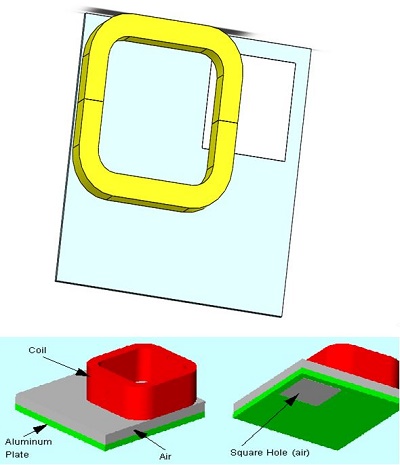
In this example, it's crucial to understand that the exciting coil forms a closed loop, making it multiply-connected. Due to the problem's asymmetry, the entire coil needs to be incorporated into the model. The current density should flow orthogonally to the entry port. To facilitate picking, the coil was divided into two parts: Coil-1 and Coil2-1. Additionally, since the entry and exit ports are the same, only the entry port needs to be specified.
| Name | Number of turns | Magnitude | Phase |
| Wound Coil | 100 | 19.39 A | 0 |
Meshing
Meshing plays a pivotal role in design analysis, as it directly impacts the accuracy and efficiency of simulations. EMS determines a global element size based on the model's geometry, volume, and surface area. The size and quality of the mesh, including the number of nodes and elements, depend on factors such as element size, mesh tolerance, and mesh control settings. During the initial analysis stages, a larger element size may be sufficient for quicker results, while a smaller size may be necessary for precision. Mesh Control, illustrated in Table 3, allows for fine-tuning mesh quality on solid bodies and faces. Figure 4 depicts the model after applying Mesh Controls.
.
Table 3 - Mesh control
| Name | Mesh size | Components /Bodies |
| Mesh control 1 | 5 mm | Plate |
| Mesh control 1 | 10 mm | Hole / Half coil 1/Half coil 2/ Airb |
Results
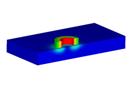
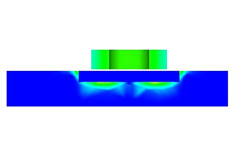
After completing the simulation for this example, the AC Magnetic Module produces a range of results crucial for electromagnetic analysis. These include Magnetic Flux Density (refer to Figures 3 and 4), Magnetic Field Intensity, Applied Current Density (depicted in Figure 5), Eddy Current Density (shown in Figure 6), Force Density, and Losses Density (illustrated in Figure 7). Additionally, a comprehensive results table is generated, containing computed parameters such as Inductance, Current, Induced Voltage, Losses, and Electromagnetic Forces. These results provide valuable insights into the electromagnetic behavior of the system under consideration.
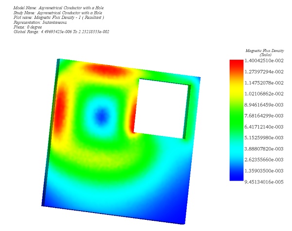
Figure 3 - Magnetic Flux Density in the plate, fringe plot (Phase 0)
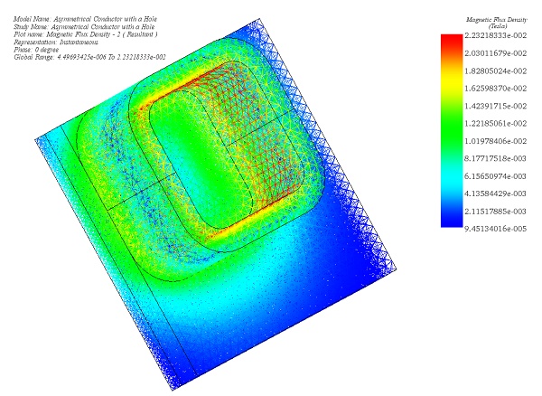
Figure 4 - Magnetic Flux Density, mesh plot (Phase 0)
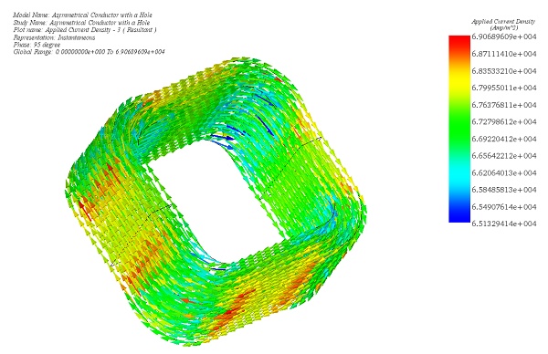
Figure 5 - Applied Current Density, vector plot (Phase 95 deg)
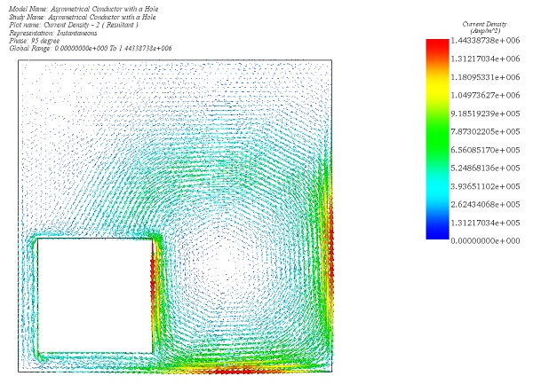
Figure 6 - Eddy Current Density in the plate , vector plot (phase 95 deg)
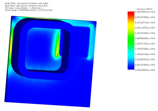
Figure 7 - Solid Loss due to the Joule Effect
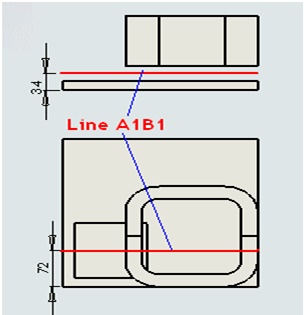
To fulfill the benchmark requirements outlined by TEAM 7, it's essential to plot the magnetic flux density (Bz) along the Z-axis through the line A1B1, as depicted in the provided sketch. This plot will provide valuable insights into the distribution of magnetic flux density within the analyzed system, enabling further evaluation and validation of the simulation results.
The measured data is reported in [1] and [2].
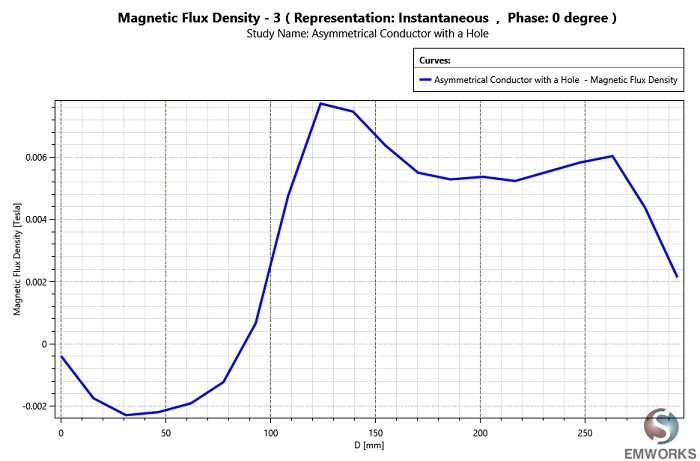
The above results compare well to the measured data reported in [1] and [2].
Conclusion
The application note delves into TEAM Benchmark 7, a pivotal study initiated at Argonne National Laboratory, focusing on numerical techniques for electromagnetic field problem-solving. It showcases a model featuring an aluminum plate with an eccentric hole and an exciting coil, emphasizing asymmetry. Critical aspects include skin depth calculations, AC magnetic analysis, material properties, meshing techniques, and result interpretation. Through EMS's AC Magnetic module, the study facilitates insightful visualizations of magnetic flux density, current density, and losses, among others. The note underscores the importance of meticulous meshing and thorough result analysis for accurate electromagnetic simulations. The findings align closely with measured data, validating the effectiveness of the approach in electromagnetic analysis, thus contributing significantly to the broader understanding of electromagnetic field problems.
References
[1] K. Fujiware and T. Nakata, "Results for benchmark Problem 7 (asymmetric conductor with a hole)," in Compel, vol. 9, no. 3, pp. 137-154, 1990.
[2]. Oszkar Biro and Kurt Preis, "An edge finite element eddy current formulation using a reduced magnetic and a current vector potential," IEEE Transactions on Magnetics, vol. 36, no. 5, pp. 3128-3130, September 2000.