Exploring Eddy-Current Testing (ECT) - A Non-Destructive Approach
Eddy-current testing (ECT) is a non-destructive testing (NDT) technique rooted in electromagnetic induction. Its primary application lies in surface inspection, aimed at detecting both surface and sub-surface imperfections within a specimen.
A single-element ECT probe comprises a conductive wire coil energized by an AC source. This coil generates an alternating magnetic field in its vicinity. Within the conductive material nearby, the coil's field induces eddy currents. These eddy currents flow in a direction that opposes the magnetic flux produced by the coil. Anomalies in the material introduce variations in electrical conductivity and magnetic permeability, subsequently altering the eddy currents and the impedance experienced by the coil.
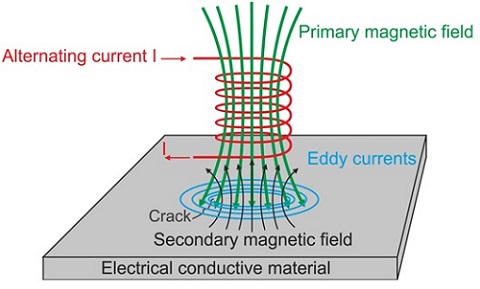
Figure 1 - Eddy Current Testing principle
Understanding Impedance Variation in ECT with Parametric Analysis
In this example, we delve into the world of eddy-current testing (ECT) where a conductor plate undergoes scanning by a coil. The key focus lies in detecting cracks on the plate by monitoring variations in the coil's impedance. By introducing different crack sizes and excitation frequencies, we gain insights into the coil's behavior across various scenarios. The accuracy of EMS results is confirmed through rigorous experimental testing.
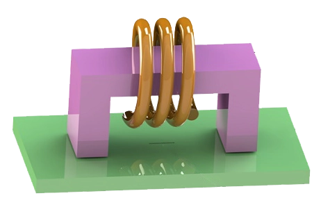
Below, you'll find a 3D representation of the simulated probe. To tackle this example, we employ a parametric AC magnetic analysis to measure the coil's impedance at various positions, with a step size of 2 mm.
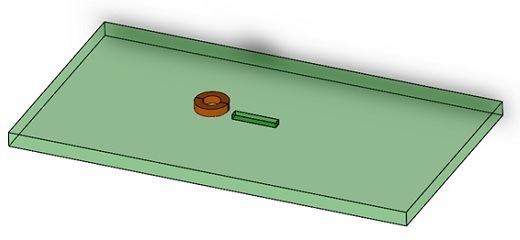
Figure 2 - CAD model of simulated NDT example
Figure 3 shows the geometrical parameters of the model. The crack width and depth are 2mm and 1.3mm respectively. Two different crack lengths have been simulated- 12 mm and 8mm.
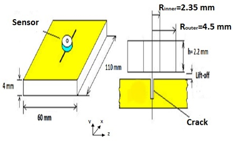
Figure 3 - Geometrical parameters of the model
Study
The EMS AC Magnetic module is a powerful tool for computing a range of results, including magnetic flux density, eddy current density, and loss density, especially for sinusoidal excitation. Additionally, EMS provides valuable data such as total eddy current loss, Joule loss, and impedance matrix. In the context of this example, a parametric analysis will be employed to obtain impedance data for each coil position.
These four steps should be followed to perform an AC Magnetic simulation in EMS:
-
Create a new AC Magnetic study
-
Apply suitable materials to the parts
-
Apply a suitable coil (either voltage or current-driven) with the correct excitation.
-
Mesh and Run the simulation
Materials
Both the coil and the plate are made of copper. Below are the properties of the copper and the air surrounding the plate and coil.
Table 1 - Copper properties
| Relative permeability | Electrical conductivity S/m | |
| Copper | 1 | 58.100e+6 |
| Air | 1 | 0 |
Coil
The sensor here is the coil. Table 2 contains the coil properties.
Table 2 - Coil properties
| Number of turns | Current magnitude | |
| Wound Coil | 170 | 20 mA |
Mesh
Mesh quality plays a crucial role in all Finite Element Method (FEM) simulations. The accuracy of results and the time required for solving are strongly influenced by the mesh size. In line with Finite Element Analysis (FEA) principles, models with finer mesh (smaller element size) tend to provide highly accurate results but may require longer computing times. Conversely, models with coarser mesh (larger element size) can yield results more quickly but with reduced accuracy. EMS simplifies mesh generation by automatically estimating the global size of the model. Moreover, EMS enhances meshing flexibility by allowing users to control mesh size on solid bodies and faces using the mesh control option. In this particular example, a mesh control is applied to the small air region surrounding the coil. The crack's air region is finely meshed, with a maximum element dimension of 0.1mm, as depicted in Figure 4.
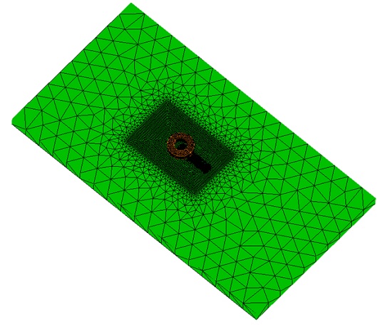
Figure 4 - Meshed Model
EMS results
Upon completing the parameterized simulation with specific parameters, including a crack length of 12mm, coil lift-off of 0.13 mm, and an excitation frequency of 50 kHz, the results are now available. EMS's parametric analysis capability empowers users to explore variations in either geometric or simulation parameters, such as current, number of turns, frequency, and mesh size. All the outcomes from different scenarios are consolidated within a single study.
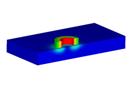
Figure 5 visualizes the current density distribution within the model in the absence of a crack. Eddy currents are concentrated within the skin depth. In Figure 6, the current density distribution is depicted when the coil is positioned directly above the center of

Figure 5 - Current density distribution in case of plate without crack
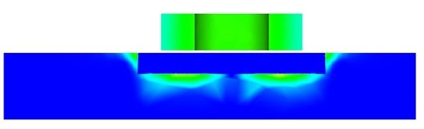
Figure 6 - Current density distribution in case of plate with crack
The coil, acting as a probe, scans the plate along the direction of the crack length. To reduce the computational complexity, symmetry is applied, simulating only half of the coil positions, starting from the crack center and moving toward its end. At each step, the impedance of the coil is measured. Figure 7 illustrates that the impedance reaches its maximum value at the center of the crack. In Figure 8, a comparison is drawn between EMS simulation results and experimental measurements [1], demonstrating a very close match between the two.
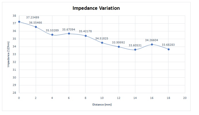
Figure 7 - Impedance variation of coil sensor
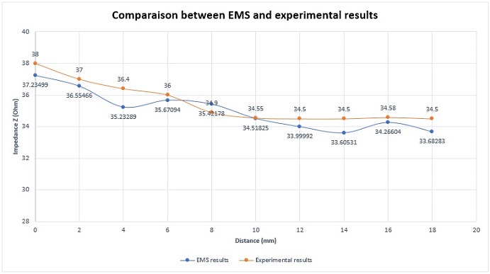
Figure 8 - Comparison between EMS and experimental results for the impedance variation (50kHz and 12 mm crack length)
Figure 9 represents the absolute change in the impedance of EMS and experimental tests. It can be calculated as shown in the formula below:
![]()
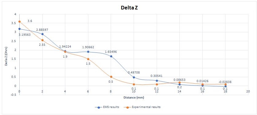
Figure 9 - Comparison between EMS and experimental results for absoluteimpedancevariation (50kHz and 12 mm crack length)
Relation between crack dimensions and captured signal
The crack size affects the impedance behaviour during the sensor scan. Figure 10 shows a comparison of the impedance variation for two different crack lengths. The variation in the impedance with higher crack length is more important and could be detected easier.
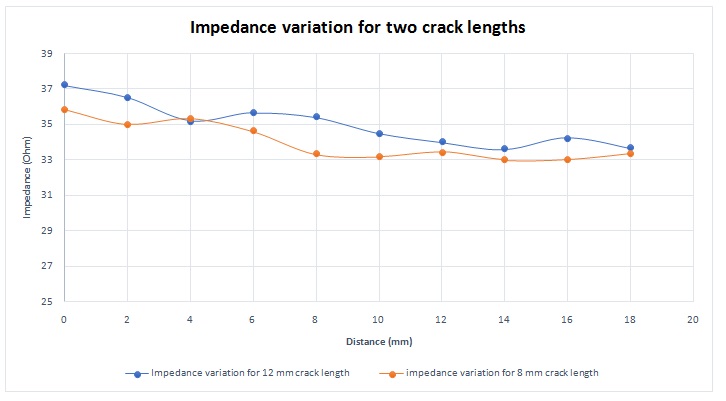
Figure 10 - Impedance variation for different crack lengths
EMS simulation results match very well the experimental results as shown in figure 11.
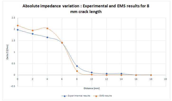
Figure 11 - Absolute impedance variation for 8 mm crack length
Relation between excitation frequency and captured signal
The coil can be excited with different frequencies. EMS and experimental results at Figure 12 demonstrate that crack detection is easier at higher frequencies. This deduction can be explained by the relationship between frequency and skin depth. The formula below shows which parameters depend the skin depth:
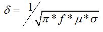
Where f is the excitation signal frequency, is the material conductivity and
is the material permeability.
The skin depth is inversely proportional to the frequency. So, a higher frequency gives a smaller skin depth. As a result, the generated eddy current will be closer to the plate surface and the sensor. A higher magnetic flux will be produced by this eddy current and will affect more the probe. Once again, EMS calculation and measured data are in very good agreement.
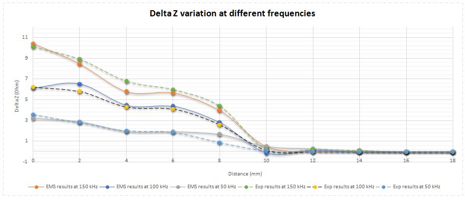
Figure 12 - EMS and Experimental results of absolute impedance variation at different frequencies
Relation between lift-off distance and captured signal
The distance between the coil sensor and the specimen surface is critical for accurate crack detection. As shown in Figure 13, the variation of the absolute impedance is a more pronounced smaller lift-off.
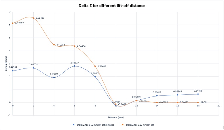
Figure 13 - EMS results of absolute impedance variation for different lift-off distance
Conclusion
This application note delves into eddy-current testing (ECT), a non-destructive technique crucial for identifying surface and subsurface flaws in conductive materials. ECT's principle, based on electromagnetic induction, allows for the inspection without direct contact, making it invaluable in sectors such as aerospace and manufacturing where safety and quality are paramount.
Using EMS's AC Magnetic module, the study showcases a parametric analysis of a conductor plate scanned by a coil to detect cracks by observing impedance variations. The simulation, focused on a plate with varying crack sizes and using different excitation frequencies, confirms EMS's accuracy against experimental data. Essential to this process are the steps of creating an AC Magnetic study, applying appropriate materials, defining coil excitation, and executing the simulation with precise mesh control.
The results reveal the impact of crack size and excitation frequency on impedance behavior, with EMS simulations aligning closely with experimental outcomes. Notably, higher frequencies enhance crack detection due to reduced skin depth, directing eddy currents closer to the surface and sensor, thereby affecting the probe more significantly. Additionally, the variation in absolute impedance becomes more pronounced with smaller lift-off distances, emphasizing the importance of sensor proximity for accurate flaw detection.
References
[1]:Hamel Meziane.2012. Etude et réalisation d ‘un dispositive de détection de défaut par méthodes électromagnétiques.