Enhancing Low-Voltage Busbar Through Electromagnetic Simulations

Used Tools:

Low Voltage Busbars

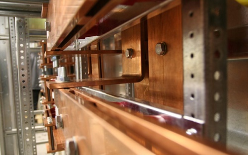
Busbars, illustrated in Figure 1, are essential electrical junctions connecting incoming and outgoing currents. They find applications in substations, aluminum smelters, and power plants. Typically made from copper or aluminum, they vary in shape based on their function and current capacity. Design considerations include managing temperature rise, ensuring energy efficiency, addressing short-circuit stresses, and facilitating maintenance.

Figure 1 - Busbars system [1]

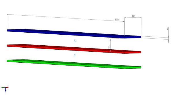
In this article, EMS will compute the Lorentz force of a low-voltage busbar system during a short-circuit scenario, comparing the results with analytical solutions. The analysis focuses on a 3-phase busbar system [1]. Below is the 3D CAD model of the simulated system, illustrating all dimensions in millimeters.

Figure 2 - The simulated model

Transient electromagnetic simulation

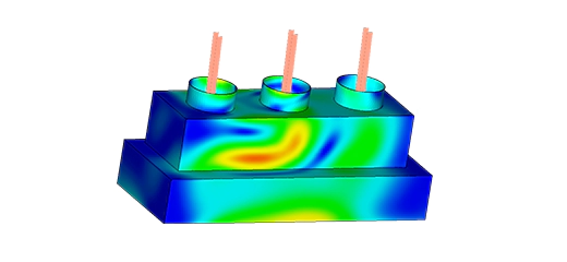
To analyze the busbars system's response during a short-circuit event, EMS's Transient module is employed. This module simulates various excitation types and generates time-domain results. The analysis includes computing Lorentz force and magnetic flux density at each conductor, compared to reference [2]. Key steps for analyzing within EMS include applying appropriate materials to solid bodies and defining boundary conditions. Each conductor, representing one phase, is modeled as a solid coil, as shown in Figure 3.

Figure 3 - Input currents

Mesh and run the model

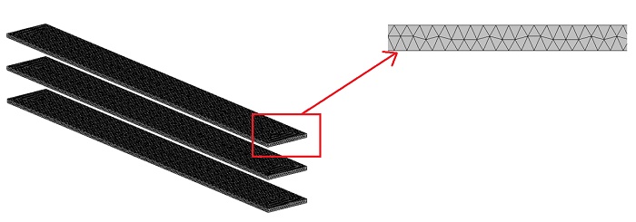
In FEM simulation, meshing impacts result accuracy and computation time. EMS uses tetrahedral elements, with total count depending on geometry dimensions. Mesh size control enhances accuracy on specific bodies or surfaces. Below is the meshed model, with 5 mm mesh control on all conductor bodies.

Figure 4 - The meshed model

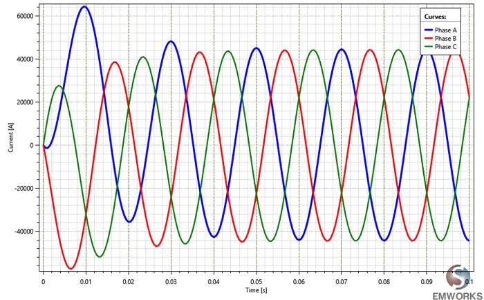
After meshing, the simulation was conducted with an analysis duration of 0.1s and a time step of 0.0005s.

Simulation Results

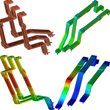
After completing the simulation, 3D plots of magnetic flux, magnetic field intensity, applied and eddy currents density, force density, and losses density versus time were generated by EMS. The results are listed in the EMS Results Table.

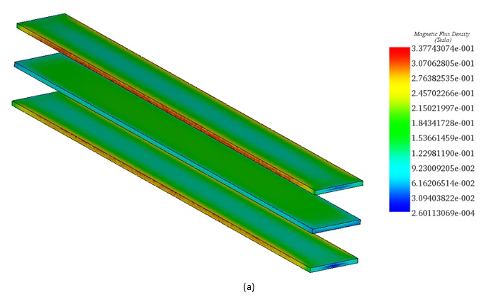
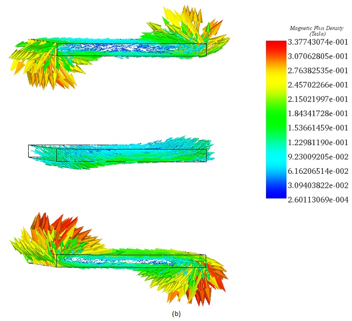
Figures 5a) and 5b) display the distribution of magnetic flux density in the busbars system at t=0.061s, revealing high spots at the edges of the conductors due to the end effect phenomenon.

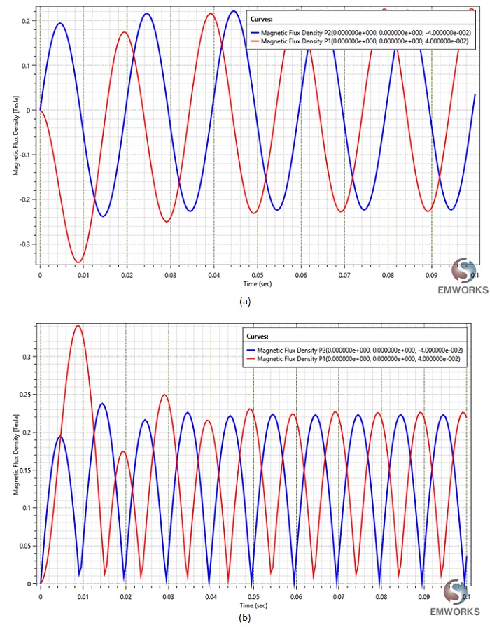
3D plot of the magnetic flux density: b) Vector plot

Figure 5 - 3D plot of the magnetic flux density: a) Fringe plot, b) Vector plot

Figures 6a) and 6b) depict the (By) component and the magnitude of the magnetic flux at points P1 and P2 (refer to Figure 2) [2]. The plots reveal that the magnetic flux density is predominantly in the Y direction, with its magnitude oscillating between 0 and 0.22T.

Figure 6 - 2D plot at two points P1 and P2 of a) (By) component of the magnetic flux density, b) The magnitude of the magnetic flux density

Figures 7 and 8 illustrate, respectively, the distribution of current density (including eddy and applied currents) and the volume of Ohmic losses within the busbars system at t=0.038s. It's observed that regions with the highest losses coincide with those experiencing the highest currents.

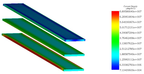
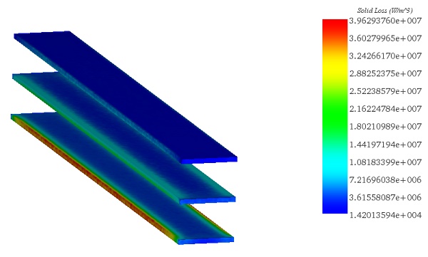
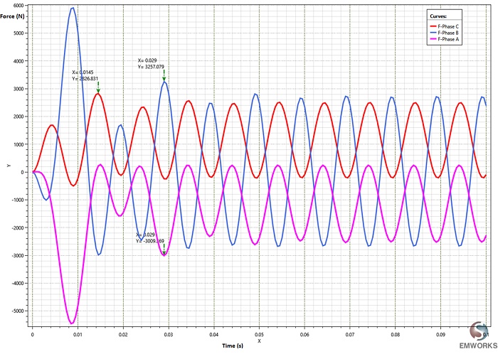
Figure 7 - Current density distribution

Figure 8 - Solid loss distribution

Figure 9 displays the Lorentz forces acting on each conductor of the busbars system over time during the short-circuit phase. Notably, all forces are directed in the Z axis, with the phase B conductor experiencing the highest electromagnetic force.

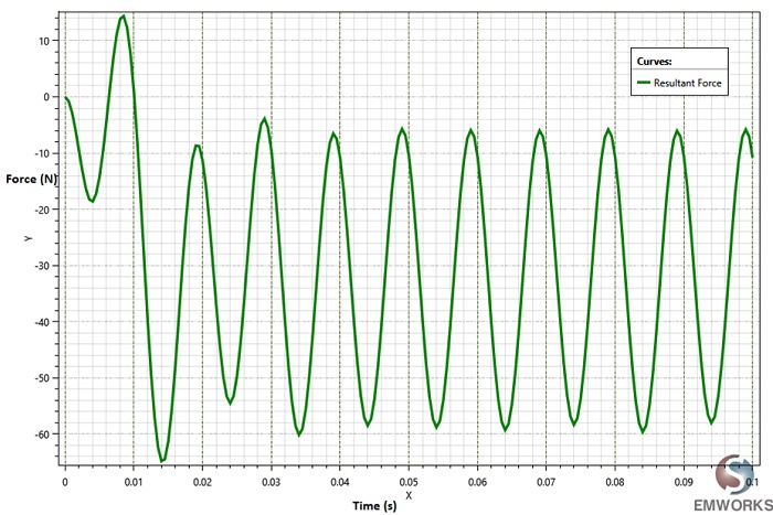
Table 1 compares the Lorentz force results obtained from EMS, analytical calculations, and reference [2]. Peak force values are selected from each phase force curve, excluding the initial oscillation, as depicted in Figure 9. Additionally, Figure 10 illustrates the cumulative forces of all three conductors, oscillating between -10 N and 60 N.

Figure 9 - Lorentz force of each conductor phase

Table 1 - Lorentz forces comparison

	EMS	Analytical _Ref [2]	Simulation _ Ref [2]	Error (EMS-Analytical) %
F_Phase A	3009.37	2945.07	2816.28	2.18
F_Phase B	3257.08	3135.13	3015.44	3.88
F_Phase C	2826.83	2945.07	2816.28	4.01

Figure 10 - Sum of the three Lorentz forces

Conclusion

In conclusion, the application note highlights the essential role of busbars as crucial electrical junctions in various industries. Utilizing EMS simulation capabilities, the article focuses on computing the Lorentz force of a low-voltage busbar system during short-circuit scenarios. By comparing results with analytical solutions, EMS demonstrates its accuracy and effectiveness in simulating complex electromagnetic phenomena.

Through transient electromagnetic simulations, EMS generates insightful data, including magnetic flux density distributions, current density profiles, and losses within the busbar system. These results provide valuable insights into system behavior, aiding in design optimization and performance evaluation.

Notably, EMS accurately predicts the Lorentz forces acting on each conductor during short-circuit events, showcasing its reliability for practical engineering analysis. Comparison with analytical calculations and reference data validates the simulation results, highlighting EMS's capability to deliver accurate and reliable electromagnetic simulations.

References

[1]: https://electropak.net/blog/manufacturing/benefits-and-uses-busbars/
[2]: Gholamreza Kadkhodaei, Keyhan Sheshyekani , Mohsen Hamzeh.Coupled electric–magnetic–thermal– mechanical modelling of busbars under short-circuit conditions. The Institution of Engineering and Technology, 2016.

Share on