Wire Bonding
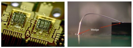
Wire bonding is a fundamental interconnection technique vital in electronics packaging, facilitating electrical contact between integrated circuits or semiconductor devices and circuit boards during fabrication. Assessing the reliability of this method in specific applications demands a comprehensive analysis integrating electromagnetic, thermal, and structural considerations.
CAD Model
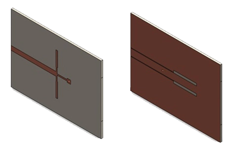
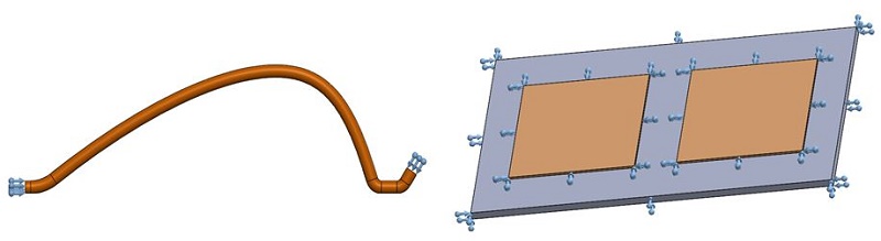
An EMS Magnetostatic simulation, coupled with thermo-structural analysis, is conducted to investigate the failure behavior of a wire bonding connection. The model under study involves a 300 µm thick wire connecting two copper layers on an aluminum substrate. The geometry of the wire loop is depicted in Figure 2a, where the height (H) represents the distance from the top of the wire to the substrate, and the bond length (L) is defined as the foot-to-foot distance (dimensions provided in Table 1). This analysis aims to ascertain the extent of wire deflection in its critical high-temperature region.
![Wire bond (H: Height, L: length) [2] a). 3D Model b).](/ckfinder/userfiles/images/Wire-bond-a%29-3D-Model-b%29.jpg)
| Dimensions | Aluminum substrate | Copper layer | Wire |
| Length(mm) | 43 | 15 | 9 |
| Height(mm) | 1 | 0.3 | 3 |
| Width(mm) | 25 | 15 | 0.3 (Diameter) |
Simulation Setup
The Magnetostatic module of EMS, integrated with steady-state thermal and structural analysis, is employed to calculate and visualize magnetic effects, temperature distribution, and mechanical deformation of the wire.
To conduct an analysis using EMS, the following crucial steps must be undertaken:
1. Material Selection: Choose suitable materials for all solid bodies involved in the analysis.
2. Electromagnetic Input Definition: Specify the necessary parameters related to electromagnetic properties.
3. Thermal Input Definition: Define thermal properties and input parameters.
4. Structural Boundary Conditions Application: Apply constraints to simulate real-world structural conditions.
5. Mesh Generation and Solver Execution: Create a mesh for the entire model and execute the solver to obtain results.
Materials
In our case study, we utilize the material properties outlined in Table 2 to characterize the materials employed in our analysis.
| Part | Density (Kg/ |
Relative permeability | Electrical conductivity (S/m) |
Specific heat capacity (J/Kg. K) |
Thermal conductivity (W/m. K) |
Elastic Modulus (Pa) |
Poisson’s ratio | Thermal expansion coefficient (/K) |
| Wire (Al-H11) | 2700 | 1 | 3.57 E+07 | 897 | 230 | 71.8 E+09 | 0.33 | 25.3 E-06 |
| Alumina substrate |
3690 | 1 | 0 | 687 | 24.7 | Not required |
||
| Copper layers | 8900 | 0.99 | 5.7 E+07 | 390 | 385 | |||
Electromagnetic Input
The wire is modeled as a solid coil carrying a direct current (DC) of 10A.
Thermal Input
The initial temperature applied to both bonded feet of the wire is set to 300 K. Additionally, for the ambient air body, the initial (ambient) temperature of the simulation is set to 300 K, and the convection coefficient on the surrounding air is set to 10 W/m² K.
Mechanical boundary condition
Fixed boundary conditions are applied to both feet of the bonded wire and to the four faces of each DCB substrate, as illustrated in Figure 3.
Meshing
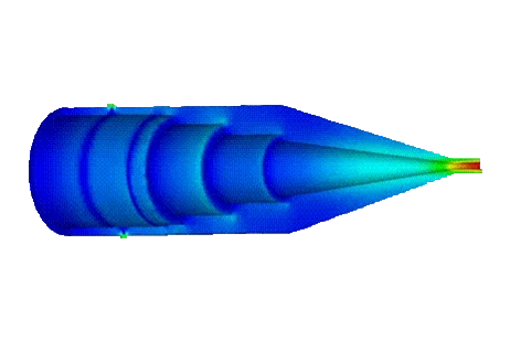
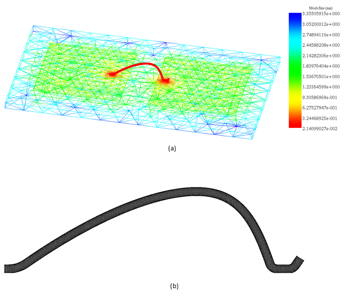
A mesh control was applied to the wire to achieve a finer mesh, given its critical role in the analysis. This finer meshing ensures greater accuracy in capturing the behavior of the wire, as depicted in Figure 4.
Results
The simulation yields various results, including magnetic flux density, magnetic field intensity, applied current density, temperature distribution, heat flux, mechanical displacement, and stress. EMS provides visualization options for these results through 3D plots and curves. For instance, the figure below illustrates the vector plot showing the distribution of applied current density between the two bonded feet of the wire.
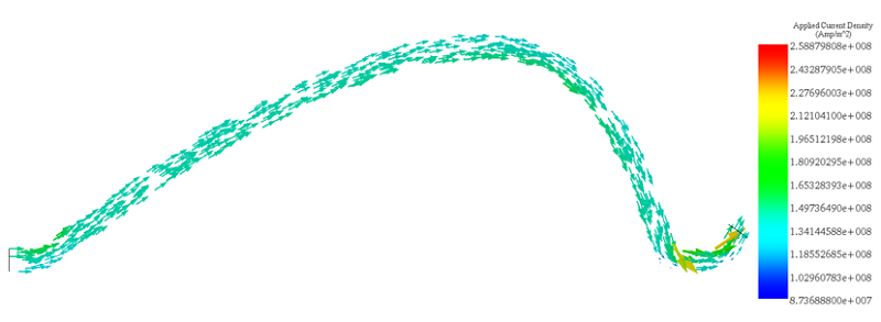
Table 3 presents the DC resistance of the simulated wire, computed and generated by EMS in the results table.
| Resistance (ohms) | |
| Solid Coil | 4.8532 E-0.003 |
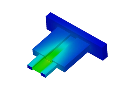
Figure 6 illustrates the temperature distribution in the wire, reaching a maximum value of 340 K.
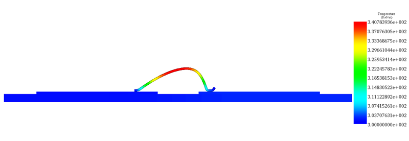
The highest temperature is concentrated at the peak point of the wire due to the concentration of current in this area. This region of elevated temperature also corresponds to the maximum mechanical deflection, as depicted in Figure 7. Table 4 presents a comparative analysis between EMS and reference results.
| EMS | Reference [2] | |
| Temperature (Kelvin) | 340 | 337 |
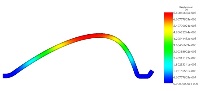
Figure 8 illustrates the displacement plot results produced by EMS for the bonded wire, showing a strong correlation with the reference results.
![The wire displacement plot along the wire - EMS and Reference [2] results](/ckfinder/userfiles/images/The-wire-displacement-plot-along-the-wire-EMS-and-Reference-%5B2%5D-results.png)
Conclusion
This application note delves into wire bonding, an essential technique in electronics packaging for establishing electrical connections between semiconductor devices and circuit boards. Utilizing EMS Magnetostatic simulation alongside thermo-structural analysis, the study examines the failure behavior of a wire bonding connection, focusing on a wire connecting copper layers on an aluminum substrate. The analysis, aimed at determining wire deflection at high temperatures, employs a comprehensive methodology incorporating material selection, electromagnetic and thermal input definition, structural boundary conditions, and precise mesh generation. The simulation's findings, visualized through 3D plots and curves, reveal critical data on magnetic flux density, temperature distribution, and mechanical displacement, emphasizing the wire's peak temperature and deflection points. Notably, the simulation results align closely with reference data, validating the model's accuracy. This study underscores the importance of integrating electromagnetic, thermal, and structural analyses to assess wire bonding reliability, offering valuable insights for optimizing electronics packaging and enhancing device performance.
References
[1]. https://www.we-online.com/web/en/wuerth_elektronik/start.php
[2]. Dagdelen, Turker. "Failure analysis of thick wire bonds. MS thesis". University of Waterloo, 2013.
[3]. Dagdelen, Turker, Eihab Abdel-Rahman, and Mustafa Yavuz. "Reliability Criteria for Thick Bonding Wire." Materials 11.4 (2018): 618.