A 3-Phase Transformer
A transformer (Figure 1) facilitates the transfer of electrical energy between circuits via electromagnetic induction, altering voltage levels as needed in power applications. Various losses occur during operation, including core losses like hysteresis and eddy current losses, and winding losses due to resistance and leakage flux. Faraday's Law dictates that transformer electromotive forces vary with flux changes over time. While ideal transformers exhibit linear behavior, real transformers experience non-linear flux behavior leading to saturation and overheating. EMS simulation of a transformer's 3D model aids in minimizing these losses, enhancing efficiency, and prolonging the transformer's lifespan.
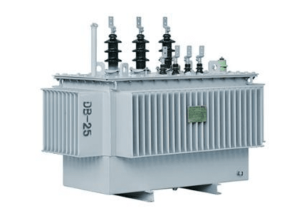
Figure 1 - Power Transformer
CAD Model
The provided example features a three-phase transformer (Figure 3) with distinct primary coils for each phase: (300 turns, 1 A/turn, 0 degrees), (300 turns, 1 A/turn, 120 degrees), and (300 turns, 1 A/turn, 240 degrees), respectively. The secondary windings are short-circuited, and both primary and secondary windings are constructed from copper. The core, crucial for magnetic induction, is crafted from laminated steel, characterized by loss. In EMS, the specification of core loss can be achieved by importing a Steinmetz (P-B) curve or defining the coefficients of a Steinmetz loss function. In this instance, importing a Steinmetz (P-B) curve is selected, considering the forthcoming AC Magnetic simulation.
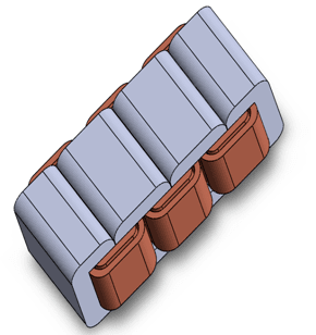
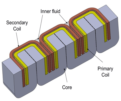
Figure 3 - 3D Model of transformer
The Study
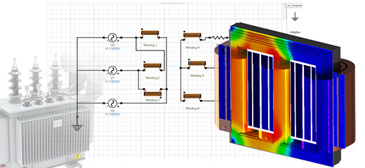
The AC Magnetic module of EMS, combined with thermal analysis, computes and visualizes magnetic fields and thermal results, addressing eddy currents, power losses, and magnetic forces. Following the coupling of an AC Magnetic study with thermal analysis in EMS, it's essential to adhere to four key steps: 1 - Apply appropriate materials to all solid bodies, 2 - Apply necessary boundary conditions (Loads/Restraints), 3 - Mesh the entire model, and 4 - Run the solver for accurate simulation outcomes.
Materials
In EMS's AC Magnetic analysis, comprehensive material properties are required for accurate simulations, as outlined in Table 1. These properties ensure a precise representation of materials in the analysis, impacting the overall accuracy and reliability of the simulation results.
| Components / Bodies | Material | Relative permeability | Conductivity (S/m) |
| Inner Coil / Outer coil | Copper | 0.99991 | 57e+006 |
| Outer Air / Inner Air | Air | 1 | 0 |
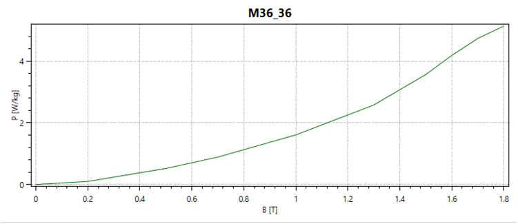
Figure 4 - Core's Material properties
Electromagnetic Input
| Name | Number of turns | Magnitude | Phase |
| Wound Coil 1 (primary) | 300 | 1 A | 0 |
| Wound Coil 2 (primary) | 300 | 1 A | 120 deg |
| Wound Coil 3 (primary) | 300 | 1 A | 240 deg |
| Wound Coil 1 (secondary) | 300 | 0 A | 0 |
| Wound Coil 2 (secondary) | 300 | 0 A | 120 deg |
| Wound Coil 3 (secondary) | 300 | 0 A | 240 deg |
Thermal Input
All air bodies in the model should be assigned as convection inputs.
Meshing
Meshing is a critical step in design analysis. EMS calculates an optimal element size based on the model's geometry, volume, and other details. The size of the mesh, determined by factors like geometry complexity and desired accuracy, influences solution speed and accuracy. Larger elements expedite approximate results, while smaller ones ensure precision. Adjusting mesh quality with mesh control enhances accuracy.
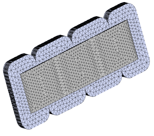
Figure 5 - Meshed Model
Results
The AC Magnetic Module coupled with thermal analysis in EMS yields comprehensive results including Magnetic Flux Density, Magnetic Field Intensity, Applied Current Density, Force Density, Losses Density, and thermal parameters like Temperature, Temperature Gradient, and Heat Flux. Table 1 contains computed parameters such as Inductance, Current, Induced Voltage, and Losses for each coil. Specifically, the induced voltage of the six coils can be found in Table 1.
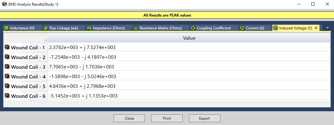
Figure 6 - Results Table
EMS provides various types of plots, including fringe and vector plots of the magnetic flux density, allowing for comprehensive visualization and analysis of electromagnetic phenomena.
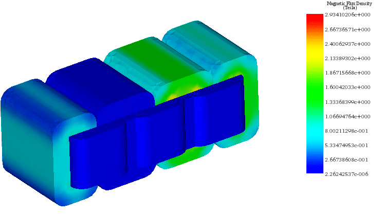
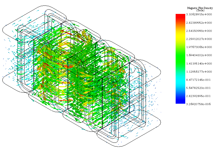
Figure 8 - Magnetic Flux Density in the core of the transformer, Phase 0 deg
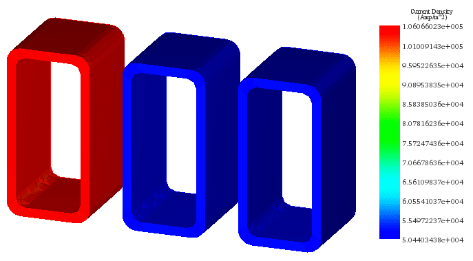
Figure 9 - Applied Current Density, Phase 0 deg
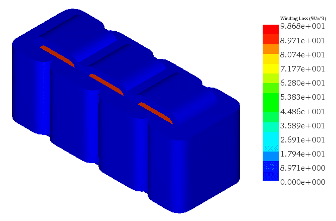
Figure 10 - Winding Losses in primary coils, line plot'
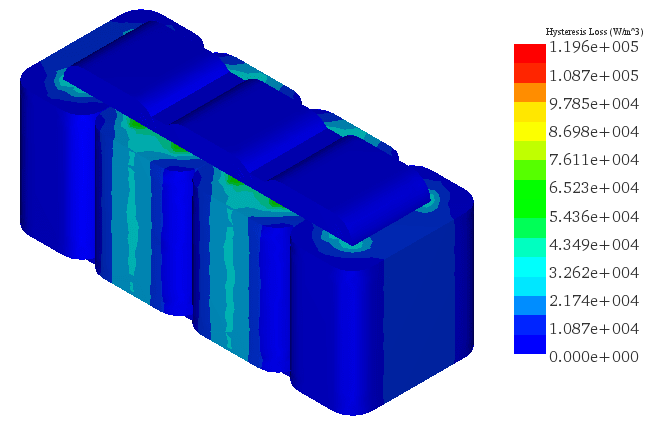
Figure 11 - Hysteresis Loss
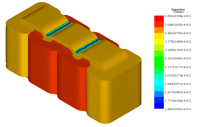
Figure 12 - Temperature in the transformer
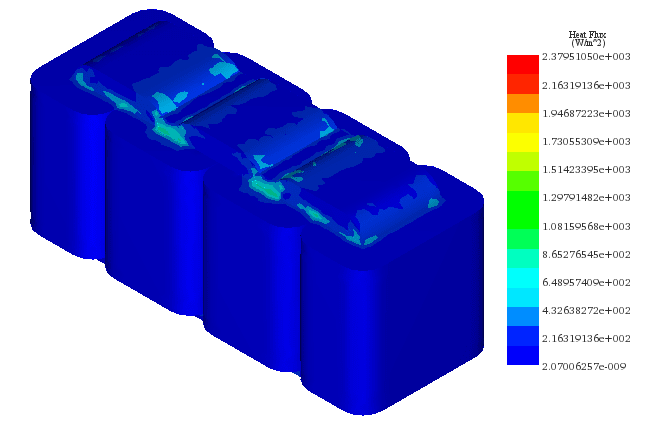
Figure 13 - Heat Flux
Conclusion
The application note on the 3-phase transformer delves into the intricacies of transformer operation and design optimization through EMS simulation. It addresses critical aspects such as losses, material properties, electromagnetic input, and thermal considerations. By employing EMS's AC Magnetic module coupled with thermal analysis, the study aims to enhance efficiency and extend the transformer's lifespan. Through detailed modeling and analysis, it offers insights into magnetic flux density, field intensity, current density, and losses within the system. By adhering to a structured simulation workflow and utilizing accurate material properties, the study provides a comprehensive understanding of transformer behavior under various operating conditions, aiding in the development of efficient and reliable power systems.