Electromagnetic-Thermal Coupling Analysis for Parallel Wires

Parallel current-carrying wires

In this illustration, we will explore the coupling analysis capabilities of EMS through a straightforward example involving two parallel wires, as depicted in Figure 1. We conducted a transient magnetic simulation coupled with thermal analysis to verify the accurate transfer of electromagnetic-induced ohmic heating to the thermal domain.

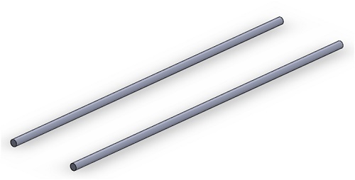
Figure 1 - CAD model of simulated example

Transient Magnetic analysis operates within the realm of low-frequency electromagnetic phenomena, where displacement currents are disregarded. This analysis specifically computes magnetic fields that undergo temporal changes, commonly triggered by current or voltage surges. It encompasses both linear and non-linear aspects, encompassing the consideration of eddy currents, power losses, and magnetic forces.
                      

Simulation setup

After creating a Transient Magnetic study coupled to thermal analysis in EMS, four important steps shall always be followed:

1. apply the proper material for all solid bodies

2. apply the necessary electromagnetic inputs

3. apply the necessary thermal inputs

4. mesh the entire model and run the solver

Materials

In Table 1, wires' material properties are listed.

Table 1 -  Material properties

Electromagnetic inputs

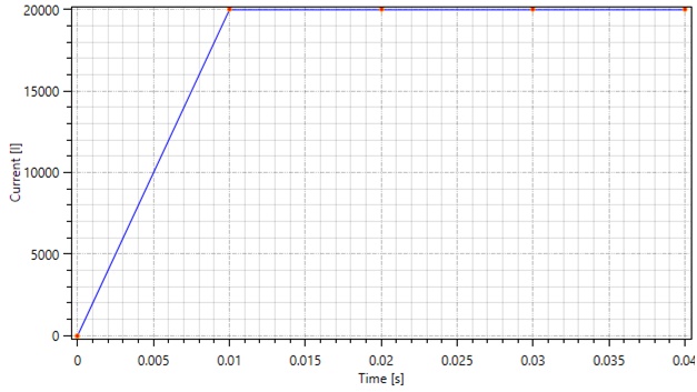
In this study, a pulse current is administered to each wire in a uniform direction. Figure 2 illustrates the waveform of the pulse excitation current.  

Meshing

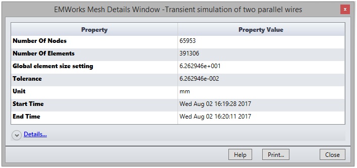
Meshing plays a pivotal role in design analysis. EMS calculates an optimal global element size for the model, factoring in its volume, surface area, and intricate geometric features. The resulting mesh size (comprising nodes and elements) is contingent upon several factors, including model geometry, dimensions, specified element size, mesh tolerance, and mesh control.
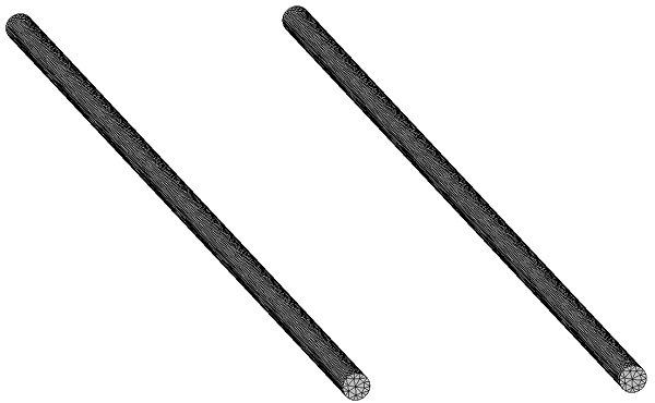
During the initial phases of design analysis, when approximate results are acceptable, opting for a larger element size can expedite the solution process. However, for greater precision, a smaller element size may be necessary. Figures 3 and 4 offer a comprehensive view of the mesh details and the finalized mesh, respectively.

 

Electromagnetic-thermal results

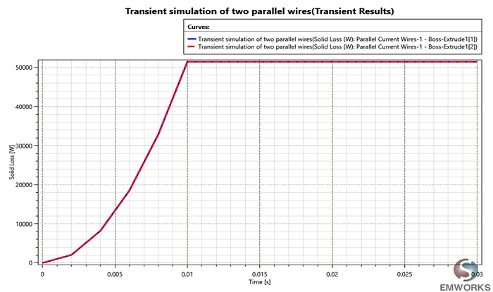
Upon completing the setup and successfully running the Transient Magnetic simulation coupled with thermal analysis, comprehensive electric and thermal transient results are generated. The total thermal solving time is configured to be 0.03 seconds, with a time increment of 0.002 seconds.
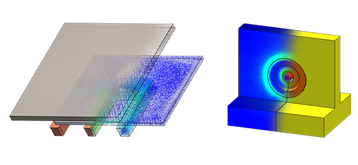
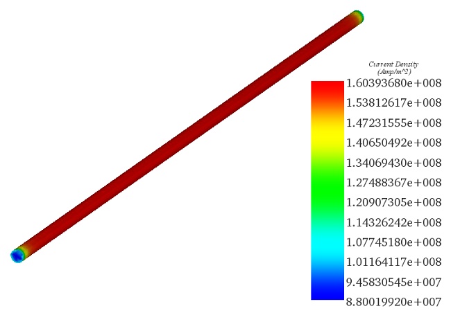
In the figure below, you can observe a 3D plot illustrating the total current density, which includes both applied and induced current, at the 0.006-second mark.
 

 

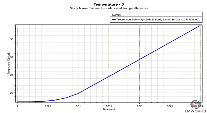
The heat generated within the two wires, referred to as solid loss, exhibits a similar evolution pattern to that of the excitation current, as depicted in Figure 6. Consequently, the temperature changes within the wires mirror the variations in solid loss, as illustrated in Figure 7. These findings align closely with the results presented in reference [1].

 

Conclusion

The application note on parallel current-carrying wires details a comprehensive analysis using EMS for coupling electromagnetic and thermal phenomena in two parallel wires. The study employs a transient magnetic simulation, disregarding displacement currents due to its low-frequency focus, to investigate temporal changes in magnetic fields caused by surges in current or voltage. This analysis is crucial for understanding linear and non-linear dynamics, including eddy currents, power losses, and magnetic forces. The simulation process involves selecting appropriate materials with specified properties for solid bodies, applying electromagnetic and thermal inputs, and meshing the model to run the solver. The material properties of the wires are outlined, along with the importance of mesh size for accurate analysis. Electromagnetic inputs are based on a pulse current with a specific waveform, and the meshing strategy is detailed for optimal analysis precision. The results showcase the effective coupling of electromagnetic-induced ohmic heating to the thermal domain, with transient electric and thermal outcomes demonstrating the temperature changes and current density distribution in the wires over time. These findings validate the simulation's accuracy in predicting electromagnetic and thermal behaviors, corroborating with the referenced benchmarks.

References

[1]: William Lawson and Anthony Johnson: “A simple Weak-Field Coupling Benchmark Test of the Electromagnetic-Thermal- Structural Solution Capabilities Of LS-DYNA Using Parallel Current Wires “