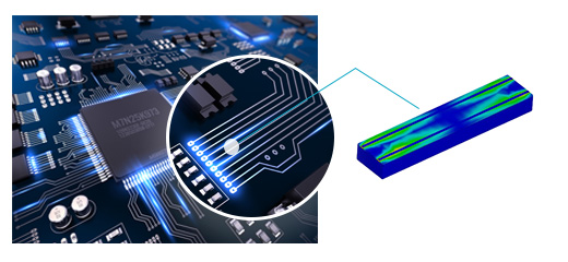
Striplines
Microstrip lines and striplines are commonly used in microwave systems. Striplines consist of a narrow metal strip on a dielectric substrate over a conducting plane.
In this validation, we analyze a strip transmission line with a dielectric substrate (?r = 12.85), infinitesimally thin conductor (w = 5mm), and 1V voltage. The substrate is enclosed within grounded shields (a = 20mm, b = 10mm) for validation against published data [1].
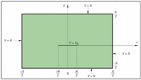
Figure 1: Cross section of a strip transmission line
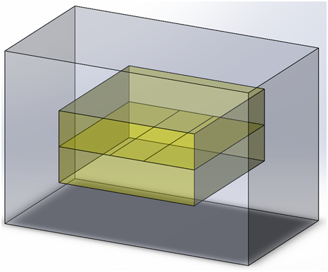
Figure 2: Solid model of the stripline
The study
EMS employs the Electrostatic module to calculate the electric potential field in the stripline and substrates. When setting up an Electrostatic study in EMS, follow three key steps: assign materials, apply boundary conditions (Loads/Restraints in EMS), and mesh the model.
Materials
In EMS Electrostatic analysis, the essential material property is relative permittivity, detailed in Table 1 for both the dielectric substrate and surrounding air.
| Component/Body | Material Name | Relative Permittivity |
| Airbox | Air | 1.0 |
| Substrate 4 | TMM-13 | 12.85 |
| Substrate 5 | TMM-13 | 12.85 |
Table 1: Relative permittivity of the two dielectric substrates and the surrounding air
The application of materials is straightforward. Just right-click on the component icon and apply the material.
Load/Restraints
Loads and restraints are crucial for defining the electric and magnetic environment of the model. They directly affect the analysis results and are applied to geometric features, automatically adjusting to changes. Here, the stripline has 1V electric potential, and the shielded conductor around the substrate is grounded.
Meshing
Meshing is a critical step in design analysis. EMS calculates the global element size, considering volume, surface area, and geometry. The size of the mesh, determined by factors like element size and tolerance, depends on model geometry and accuracy needs. For this benchmark, a 3 mm global element size with a 0.15 mm mesh tolerance is used. To enhance accuracy in regions with significant field variations, a 1.2 mm local mesh control is applied to the dielectric substrate. See Figure 3 for the mesh.
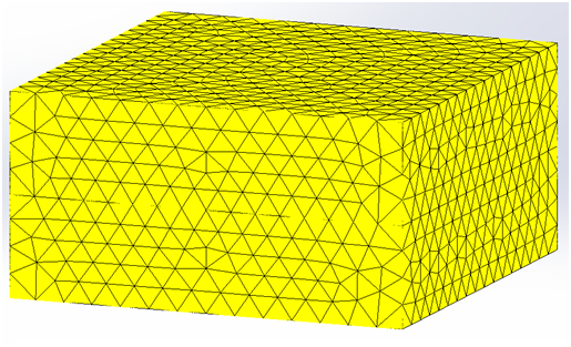
Figure 3: Mesh of the structure without the air region
Results
After a successful run, the Electrostatic module generates four result folders and a result table. These folders contain data for electric field E, displacement field D, potential distribution V, and force density, while the table includes energy data. You can visualize these results in various formats such as fringe, vector, contour, section, line, and clipping plots. These visualizations can be zoomed in, exported, and analyzed. In this benchmark, we compare the 3D electric potential field plot with the results in [1]. Additionally, we use EMS's line plot feature to compare electric potential at three points: (10, 3.75), (11.558, 3.75), and (12.338, 1.25). Figures 4-6 show that EMS results align with those reported in [1].
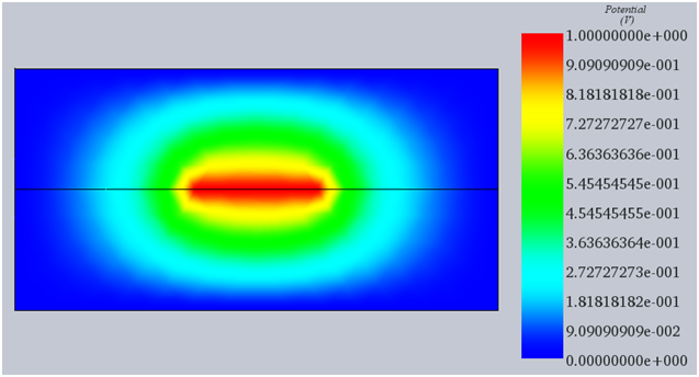
Figure 4: Electric potential field obtained by EMS
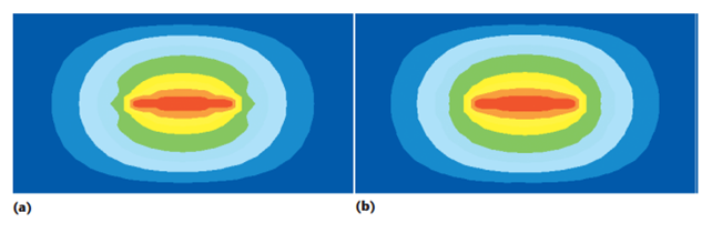
Figure 5: The results of the electric potential field using (a) the DBEM and (b) the FEM as reported in [1]
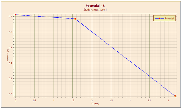
Figure 6 : Line plot of the electric potential between (10, 3.75), (11.558, 3.75) and (12.338,1.25) obtained by EMS
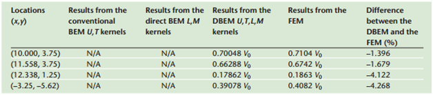
Table 2: The results of electric potential under diverse numerical methods reported in [1]
The results from the 3D electric potential plot and the magnitudes of the reference points (Point 1: 0.7112 V, Point 2: 0.6849 V, Point 3: 0.1867 V) as a ratio to the maximum potential V0 (1V) on the stripline closely align with the findings in [1].
Conclusion
This application note provides a comprehensive validation study of a strip transmission line using EMS, focusing on electrostatic analysis to understand the electric potential field within a stripline configuration. The study meticulously sets up a simulation environment for a strip transmission line with specific geometric and material parameters, notably a dielectric substrate with a relative permittivity of 12.85, grounded shields, and an applied voltage of 1V. Key steps in the EMS simulation process include material assignment, application of loads and restraints, and detailed meshing to ensure accurate representation and analysis. The results, demonstrated through various data visualization formats, indicate a successful alignment of EMS findings with previously published data, showcasing the tool's efficacy in electrostatic problem-solving. The precise calculation of electric potential fields and the validation against established benchmarks underscore EMS's capabilities in addressing complex electrostatic challenges in microwave system design, offering valuable insights for engineers and researchers in the field.
References
[1] Chyuan, S.W.; Liao, Y.S., Chen, J.T.; "An Efficient Method for Solving Electrostatic Problems," Computing in Science and Engineering, Vol. 5, No. 3, May-June 2003, pp. 52-58