Academic Learning Examples

Understanding Magnetic Field Strength Calculation for Cylindrical Coils

Used Tools:

Physics

A cylindrical coil is employed to generate a robust magnetic field within a specific domain. The coil achieves this by winding the same wire multiple times around a cylindrical structure, amplifying the magnetic field's strength. The term "N" represents the number of loops or turns the cylindrical coil contains, with a higher number of turns resulting in a more potent magnetic field.

Our objective is to calculate the magnetic field strength, denoted as "B," at a point "P" situated along the axis of a cylindrical coil. This coil possesses certain characteristics, including a length "L," radius "R," "N" turns, and it carries an electrical current "I." As per the Biot-Savart law, the magnetic field generated by a current loop is determined by the following formula:

$d B subscript Z equals fraction numerator mu subscript 0 R squared space d i over denominator 2 r cubed end fraction$

Where $mu subscript 0 equals 4 pi cross times 10 to the power of negative 7 end exponent space H divided by m space$ is the vacuum permeability.

Schematic of a cylindrical coil

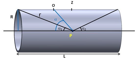
Figure 1 - Schematic of a cylindrical coil

To calculate the total magnetic field on the axis of the cylindrical coil, we need to consider the contributions from all the individual loops within the coil. To do this, we can divide the length of the cylindrical coil into small elements of length "dz" to sum up the magnetic fields from each of these elements.
The number of coil turns contained within a length "dz" space can be calculated as follows:

$fraction numerator d N over denominator d z end fraction equals N over L$

Therefore:

$d N equals N over L d z$

The total current in a length $d z space$ is:

$d i equals I d N equals I N over L d z$

The magnetic field contribution $d B$ at point $P space$ due to each element $d z$ carrying current $d i space$ is:

$d B subscript Z equals fraction numerator mu subscript 0 space R squared over denominator 2 space r to the power of 3 space end exponent end fraction I space N over L d z space space space space space left parenthesis 1 right parenthesis$

For each element of length $d z space$ along the length of the cylinder, the distance $z space$ and the angle $alpha space$ change, while the value of $space R space$ remains constant.From figure 1 we have:

$r space equals fraction numerator R over denominator sin left parenthesis alpha right parenthesis end fraction$

and

$cos space alpha equals negative z over R space space space space space left parenthesis 2 right parenthesis$

Expression (2) can be differentiated as:

$negative fraction numerator d alpha over denominator sin squared alpha end fraction equals negative fraction numerator d z over denominator R end fraction$

Which results with:

$d z space equals fraction numerator R space d alpha over denominator sin squared alpha end fraction$

Formula for $d z space$ and formula for $space r space$ can be substituted in the equation (1):

$d B subscript Z equals fraction numerator mu subscript 0 space end subscript I space N space sin alpha over denominator 2 space L end fraction d alpha$

Total magnetic field $B subscript z$ at any point on the axis can be obtained by integrating from $alpha subscript 1$ to $pi minus alpha subscript 2$ :

$B subscript z equals space contour integral subscript alpha subscript 1 end subscript to the power of pi minus space alpha subscript 2 end exponent space space fraction numerator mu subscript 0 space I space N space sin alpha over denominator 2 space L end fraction d alpha equals fraction numerator mu subscript 0 space I space N over denominator 2 space L end fraction contour integral subscript blank subscript alpha subscript 1 end subscript end subscript to the power of pi minus alpha subscript 2 end exponent space sin space alpha space d alpha equals fraction numerator mu subscript 0 space I space N over denominator 2 space L end fraction left parenthesis cos space alpha subscript 1 plus cos space alpha subscript 2 right parenthesis$

$B subscript z equals fraction numerator mu subscript 0 I space N over denominator 2 space L end fraction left parenthesis cos space alpha subscript 1 plus cos space alpha subscript 2 right parenthesis space space$

Hence this expression gives the magnetic field at point on the axis of a cylindrical coil of finite length.

Model

A cylindrical coil with the following specifications: length 200mm, radius 5.5 mm, 100 turns, and carrying a current of 10 A, is modeled and simulated using Magnetostatic study 1 in EMS. In the simulation, copper is assigned as the material for the cylinder body, while air is used to represent the inner air of the cylinder and the rest of the assembly.
To ensure accurate magnetic field results, it is important to create a sufficiently large air domain. If you need guidance on how to assign materials in EMS, you can refer to the example titled "Computing capacitance of a multi-material capacitor." Additionally, if you want to learn how to define the air domain in EMS, you can consult the example titled "Electric field inside the cavity of a charged sphere."

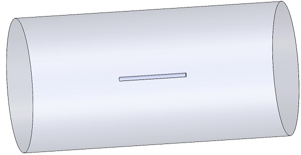
Solidworks model of the studied example
Figure 2 - CAD model of the studied example

Coil

To consider the magnetic field along the axis of the cylindrical coil, you should define a "Wound Coil" in EMS. This coil should have 100 turns and an RMS current magnitude per turn of 10A.
To apply the EMS Coil feature to the cylinder, you'll need to access its cross-sectional surface. Therefore, it's necessary to split the cylinder part into two bodies. If you need instructions on how to perform this split, you can refer to the example titled "Magnetic field on axis of a current loop."
Figure 3 in the documentation displays the Entry and Exit ports of the Coil. In this particular case, the Exit port is the same as the entry port. For detailed guidance on how to define the Wound Coil, you can review the example titled "Force in a magnetic circuit."

Entry and Exits ports of the Coil

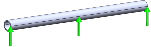
Figure 3 - Entry and Exits ports of the Coil

Mesh

Meshing plays a vital role in EMS simulations, and achieving quality meshing in both the inner air region and the cylinder is crucial for accurate magnetic field calculations. To maintain accuracy without significantly increasing the total number of mesh elements, it's recommended to apply a mesh control with a 0.75 mm element size.
For step-by-step instructions on how to apply this mesh control, you can refer to the example titled "Force in a magnetic circuit."

Results

To display the variation of the magnetic field along the axis of the cylinder, before running the simulation:

In the Assembly, Select the ZX plane and sketch a line along the z axis (axis of the coil), with a length equal to the length of the coil.
Then Insert/Reference geometry/Point and add a Reference point for each end of the line.
In the EMS feature tree, right click study and select Update geometry .
Mesh and run the study.

Once the simulation is complete:

In the EMS feature tree, Under Results , right click on the Magnetic Flux Density folder and select 2D Plot then choose Linear.
The 2D Magnetic Flux Density Property Manager Page appears.
In the Select points tab, click Import.
Click OK .

The theoretical and EMS result of the magnetic flux density along the axis of the cylindrical coil are plotted in Figure 4.
It’s obvious that EMS result comply with the Biot-Savart law.

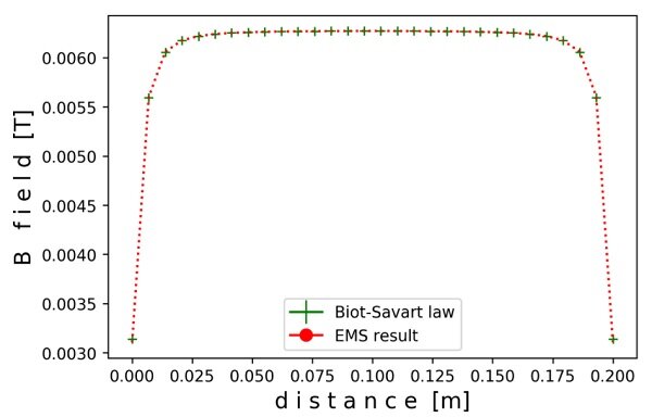
Figure 4 - Comparison of EMS and theoretical results for magnetic flux density along the axis of a cylindrical coil

Conclusion

This application note delves into the computation of the magnetic field strength "B" along the axis of a cylindrical coil, guided by the Biot-Savart law. It meticulously derives a formula for calculating the magnetic field produced by a cylindrical coil, characterized by its number of turns "N", length "L", radius "R", and the electric current "I" it carries. This derivation involves segmenting the coil into infinitesimally small sections to aggregate the magnetic contributions from each, culminating in an integrated expression for the total magnetic field at any axial point.

The practical exploration of the study is illustrated through the modeling of a cylindrical coil specified with a length of 200mm, radius of 5.5mm, 100 turns, and carrying a current of 10A. The simulation, executed using a Magnetostatic study tool, underscores the significance of precise meshing and the establishment of an adequately large air domain for accurate magnetic field assessments. The modeling process includes defining a "Wound Coil" feature, essential for accurately capturing the coil's magnetic field along its axis.

Results are presented through a process that visualizes the magnetic field variation along the coil's axis, providing a detailed guide for generating a 2D plot of the magnetic flux density. The comparison between simulation results and theoretical calculations derived from the Biot-Savart law affirms the simulation model's accuracy, illustrating the tool's adherence to physical laws.

Download Application Model

Share on