Switched Reluctance Motors
Switched reluctance motors (SRMs) are gaining popularity across industries for their simplicity and efficiency. This note explores modeling an SRM using EMWorks2D software, and analyzing static and on-load performance. Insights include flux linkage, field mappings, and torque analysis, highlighting EMWorks2D's effectiveness in motor design.
Description of the SRM Geometry under Study
The switched reluctance motor depicted in Figure 1 is distinguished by its configuration of 8 stator poles and 6 rotor poles. It embodies the fundamental characteristics of switched reluctance machines, known for their straightforward and uncomplicated design.
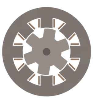
Fig. 1. 2D Cross Section of the SRM Under Study
The windings are wrapped around the stator teeth, yet their excitation occurs exclusively when they align with the rotor poles. To encompass the model geometry, an outer air volume is introduced, along with a band that encloses the rotary components, including the rotor and shaft. These additions are made in preparation for conducting transient simulations.
Key dimensions of the studied switched reluctance motor are detailed in Table 1.
| Dimension name | Dimension values in mm |
|---|---|
| Outer stator diameter | 94 |
| Inner stator diameter | 50 |
| Outer rotor diameter | 49 |
| Inner rotor diameter | 8 |
| Outer air region diameter | 188 |
| Outer band diameter | 49.5 |
| Stack length | 100 |
Definition of the SRM Materials
Defining the materials for the different components that make up the switched reluctance motor is a vital initial step in establishing the FEA-based study before initiating the simulation. Table 2 provides an overview of the materials used in the 2D geometry of the SRM, and these materials are consistent across both case studies outlined in this application note.
| SRM Part | Material |
|---|---|
| Stator poles | M27 |
| Stator windings | Copper |
| Rotor poles | M27 |
| Shaft | Stainless Steel |
Assigning Phasors to Stator Windings
Switched reluctance motors exhibit a phase count determined by the combination of stator and rotor poles. Electronic devices monitor the current switching in the SRM's various phasors, allowing for synchronized current flow with rotation [3].
In the simulated SRM, featuring 8 stator poles and 6 rotor poles, there are a total of 4 phases denoted as A, B, C, and D. The winding arrangement corresponding to these phases is depicted in Figure 2.
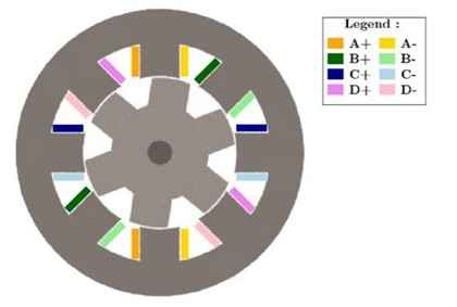
Fig. 2. Winding Configuration of the SRM Under Study, Rotation angle=90 Degrees
About the Outer Air and Band
Before embarking on the transient study within EMWorks2D, it's essential to consider two crucial elements:
-
The Outer Air region, is represented by a circular surface surrounding the SRM geometry.
-
The band part, is depicted as a circular surface encompassing the rotating components, including the rotor geometry and the shaft.
Both of these components are visually outlined in Figure 3 for reference.
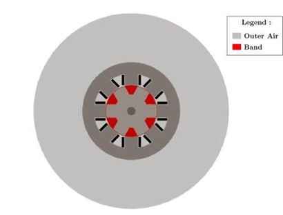
Fig. 3. Outer Air Region and Band Definition of the SRM Under Study
About the Rotor Angle
Before conducting the transient study in EMWorks2D, the user needs to define a rotor angle, a key parameter that influences the simulated motor's rotation direction. Figure 4 visually demonstrates the concept of the rotor angle. This angle is established as a global variable within the design tree during the 2D model phase. Importantly, it is utilized in both static and on-load case studies, as they both pertain to transient analyses.
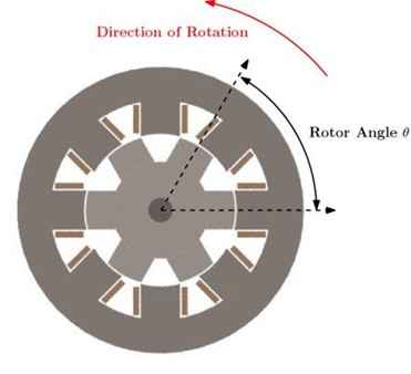
Fig. 4. Rotation Angle and Direction of the SRM Under Study
Static Analysis of the SRM: Study Parameters
In this investigation, the switched reluctance motor has been subjected to simulation at a constant speed of 1000 rpm. Furthermore, the simulation's temporal parameters, including the start time, step time, and end time, are detailed in Table 3. It's noteworthy that this study's unique characteristic is that only phase A is energized throughout the entire duration. Consequently, the SRM's output results are presented for a specific motor position.
| Defined simulation time | Time in seconds |
|---|---|
| Start simulation time | 0 |
| Step simulation time | 0.001 |
| End simulation time | 0.01 |
On-load Analysis of the SRM: Study Parameters
In this examination, the switched reluctance motor has been subjected to simulation at a consistent speed of 166.67 rpm. Additionally, the associated simulation start time, step time, and end time can be found in Table 4. Notably, this study differs from the static analysis in that all phases are activated, resulting in motor rotation. Consequently, the output results are provided for various rotor positions in this dynamic study.
| Defined simulation time | Time in seconds |
|---|---|
| Start simulation time | 0 |
| Step simulation time | 0.001 |
| End simulation time | 0.06 |
Static Study: Output Results
In the static analysis, only phase A was energized with a constant current of 20 A throughout the specified simulation duration.
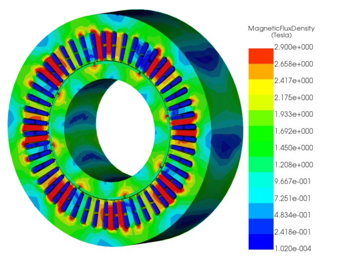
A. Field Distribution of the SRM The field distribution of the SRM when phase A is energized in the static analysis, as depicted in Figure 5 and generated using EMWorks2D, reveals that the field lines originate from the rotor poles and connect to the stator teeth associated with the excited phase. Consequently, the greatest field density magnitude (3.58 T) is observed in the stator teeth facing the rotor poles, as displayed in Figure 5.
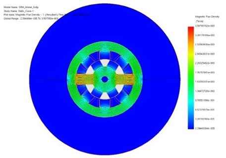
Fig. 5. Field Distribution of the SRM Under Study, Case of Static Analysis
B. Flux Linkage of Phase-A versus time
The flux linkage of phase A has been graphed over time using EMWorks2D, as shown in Figure 6. It is evident that there is a decrease in the flux linkage values from time 0 to 0.005 seconds, which corresponds to the first half of the simulation duration, followed by a subsequent increase. The time point at 0.005 seconds indicates that the rotor is in a completely unaligned position relative to phase A.
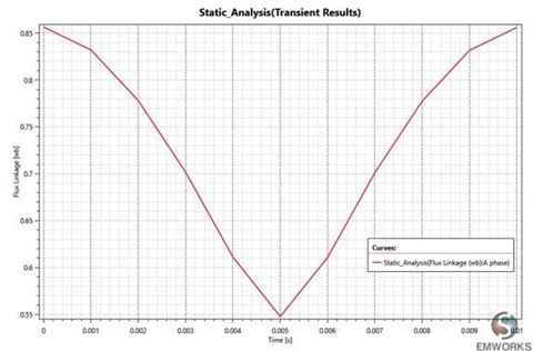
Fig. 6. Flux Linkage of the SRM Under Study, Case of Static Analysis
On-Load Study: Output Results
In the on-load analysis, all four phases were sequentially excited. The input current is depicted in Figure 7. Each phase is excited individually, aligning the rotor poles with the stator poles. To represent this, pulse excitation is employed in EMWorks2D, with each pulse having a maximum magnitude of 20 A.
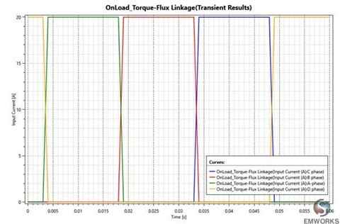
Fig. 7. Excitation of the SRM Phases, Case of On-Load Analysis
A. Field Distribution of the SRM
Let's examine the initial angle position where phase D is first excited, as depicted in the current configuration shown in Figure 7. This results in the field distribution shown in Figure 8. Only the flux lines corresponding to the rotor poles in front of the stator teeth wound with phase D coils are present. As a result, there is a higher field density (2.38 T) in the stator and rotor poles facing each other.
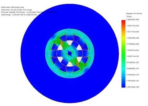
Figure. 8. Field Distribution of the SRM, Case of On-Load Analysis
B. Flux Linkage of the Phases Versus Time
The flux linkage versus time has been simulated and plotted using EMWorks2D, as depicted in Figure 9. The flux linkage waveforms of the phases exhibit a discontinuous conduction mode, corresponding to a defined period of excitation for each phase.
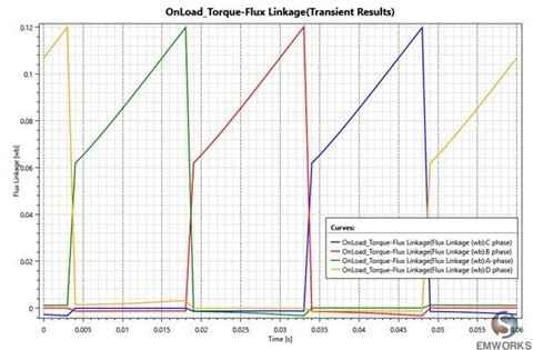
Fig. 9. Flux Linkage Versus Time, Case of On-Load Analysis
C. On-Load Torque Versus Time
The on-load torque versus time has been plotted using EMWorks2D, as depicted in Figure 10. This curve illustrates an average torque value of 2.4 Nm and a maximum torque value of 2.7 Nm for the pulse input current shown in Figure 7, with a maximum current value of 20 A. It's important to note that the torque vs. time curve in Figure 10 corresponds to a defined frequency of 8.33 Hz.
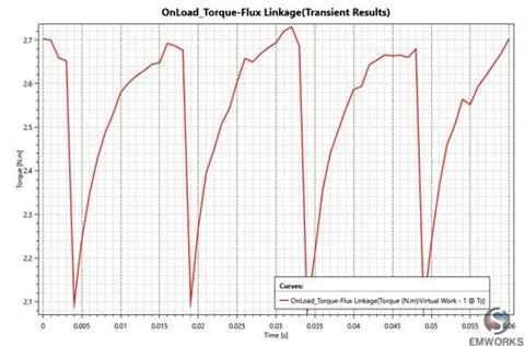
Fig. 10. On-Load Torque Versus Time, Case of On-Load Analysis
Conclusion
This study was conducted using EMWorks2D software. Initially, a straightforward structure of an 8-stator pole/6 rotor pole switched reluctance motor was designed. Subsequently, FEA-based analyses were carried out using EMWorks2D. This showcases the software's proficiency in conducting various case studies related to switched reluctance machines.
References
[1] Ahn, Jin-Woo and Lukman, Grace Firsta, "Switched reluctance motor: Research trends and overview", CES Transactions on Electrical Machines and Systems, vol.2, n. 4,p 339--347, 2018.
[2] Kehui, "Switched reluctance motor applications", Website https://www.kehui.com/products/switched-reluctance-driver-srd-system-2/.
[3] Wikipedia, "Switched reluctance motor", Website https://en.wikipedia.org/wiki/Switched_reluctance_motor.