
Electromagnetic Applications Across Industries
Accessible Electromagnetic Technology
All Applications
Biomedical
Use EMWorks to model biomedical devices, coils, and implants inside anatomical structures. Analyze SAR, field distribution, heating, and exposure limits to improve safety and performance before clinical testing.
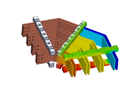
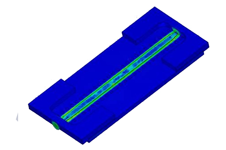
Bus Bars
EMWorks provides 3D electromagnetic tools to design high-current busbars, calculate current density and losses, and verify clearances and mechanical limits before prototyping.
Capacitors
Use EMWorks to model capacitors of any shape—parallel plate, coaxial, busbar, and custom 3D structures. Extract capacitance, visualize electric fields, evaluate parasitics, and estimate breakdown limits before building hardware.
Chip Package Board systems
Use EMWorks to simulate chip-package-board systems on full 3D geometry. Analyze signal integrity, power integrity, crosstalk, and return paths so you can optimize high-speed channels and PDNs before fabrication.
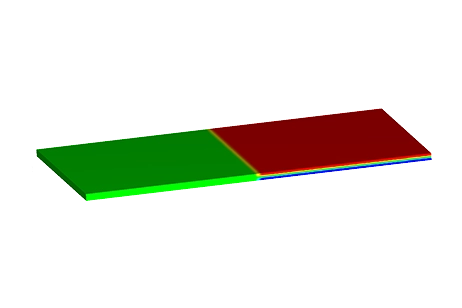
Conductors and Resistors
Simulate conductors and resistors in 3D to predict resistance, current density, Joule losses, and temperature for power and electronics applications.
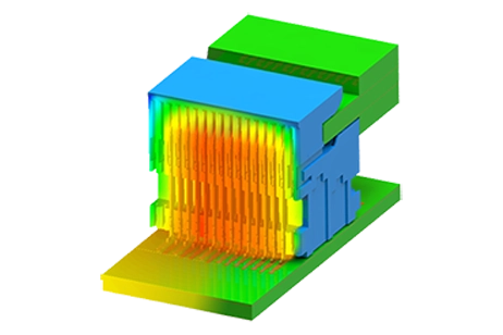
Connectors and Transitions
Analyze RF and microwave connectors and transitions with 3D EM simulation to evaluate S-parameters, impedance matching, and field distribution, improving signal integrity and minimizing loss before hardware builds.
Eddy Current Brakes
Use EMWorks to model eddy current brakes directly on your 3D geometry. Compute braking torque versus speed, analyze losses and temperature rise, and compare materials and coil configurations so you can meet performance and safety targets with fewer prototypes.
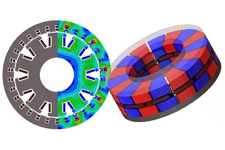
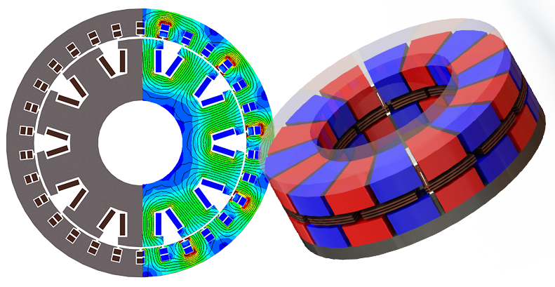
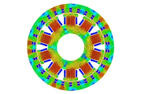
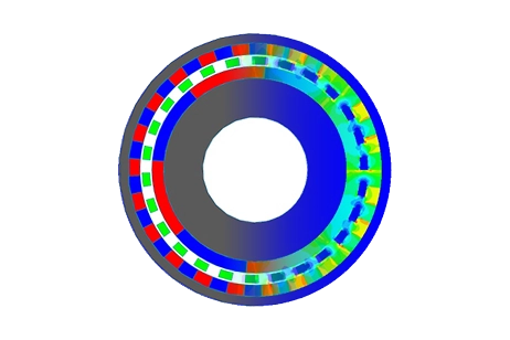
Electric Motors
Use EMWorks to model PMSM, induction, BLDC, SRM, and other machines on full 3D geometry. Evaluate torque, cogging, losses, efficiency, and temperature so you can refine slots, windings, and magnets before prototyping.
Electro-thermal
Use EMWorks to couple electrical and thermal physics on full 3D geometry. Compute Joule losses, temperature rise, hotspots and cooling performance in components and systems.
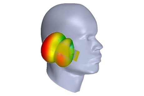
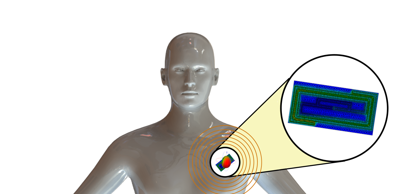
EM Exposure
Use EMWorks to model EM exposure from handheld devices, antennas, and implants in realistic anatomical models. Compute SAR, field distribution, and temperature rise to check compliance with safety limits before clinical or human testing.
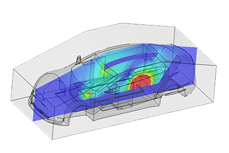
EMI/ EMC
Use EMWorks to model enclosures, PCBs, cables, and connectors. Evaluate radiated and conducted emissions, coupling paths, shielding effectiveness, and filter options so you can address EMI/EMC risks before costly compliance testing.
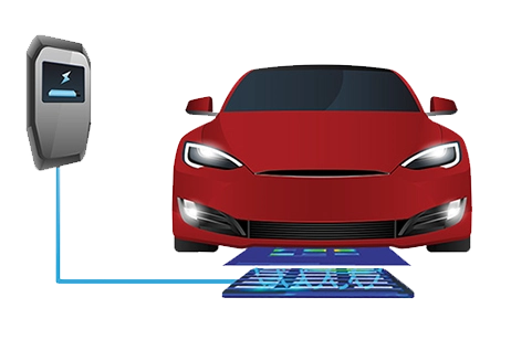
EV Battery Charging
Use EMWorks to model EV battery chargers directly on your 3D geometry. Evaluate efficiency, losses, thermal limits, fields and EMC so you can meet performance and safety targets with fewer prototypes.
Filters
Discover EMWorks’ RF and microwave filter design tools, combining full-wave EM simulation with parametric sweeps to hit tight specs for bandwidth, insertion loss, and isolation before fabrication.
Generators
Use EMWorks to model synchronous, permanent-magnet, and induction generators. Evaluate voltage, efficiency, losses, torque ripple, and temperature so you can refine slots, windings, and magnets before prototyping.
High Power Cables
Use EMWorks to model high-power cables in 3D, compute current density, losses, temperature rise and insulation stress, and compare design options.
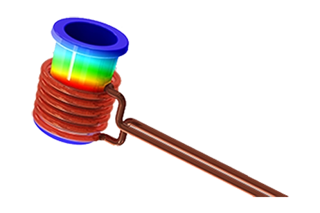
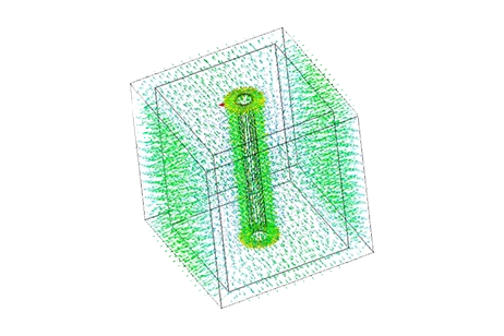
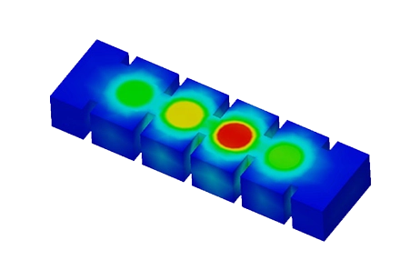
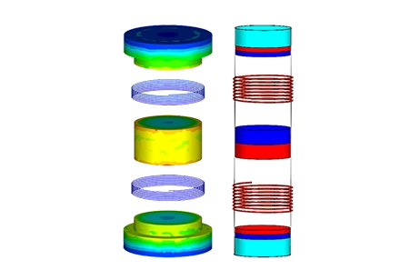
Induction Heating
EMWorks provides 3D induction heating simulation to model coils, workpieces, fixtures, and cooling. Evaluate current density, losses, and temperature rise to improve efficiency, avoid hotspots, and size power supplies before prototyping.
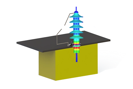
Insulators
Evaluate electric field distribution, insulation stress, creepage and clearance, and breakdown risk in high-voltage busbars, cables, surge arresters, switchgear, and insulators.
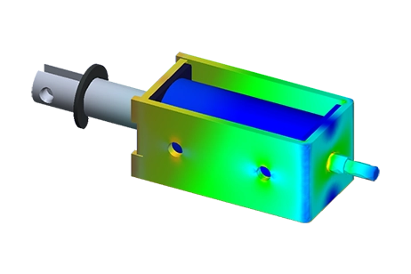
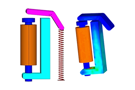
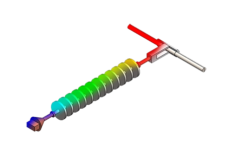
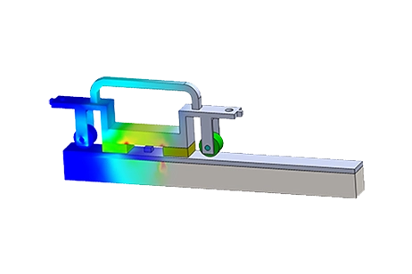
Linear and rotational actuators
Use EMWorks to model linear and rotary solenoids, voice-coil actuators, and custom mechanisms on your 3D/2D CAD. Evaluate force, stroke, current, heating, and dynamics before building prototypes.
Magnetic Gears
Use EMWorks to model coaxial, axial, and other magnetic gear topologies in full 3D. Predict transmitted torque, torque ripple, losses, efficiency, and eddy currents so you can refine pole counts, magnet arrangements, and clearances before prototyping.
Magnetic Levitation Vehicles
Use EMWorks to model magnetic levitation vehicles and sub-systems on full 3D geometry. Compute levitation force, guidance, stability, losses, and thermal limits so you can refine magnets, coils, and tracks before building prototypes.
Magneto-structural
Use EMWorks to couple magnetic fields with structural mechanics. Compute electromagnetic forces, stresses, deformation, and vibration in actuators, sensors, loudspeakers, and other devices so you can validate strength and performance before testing.
MEMS
Use EMWorks to model MEMS sensors and actuators directly on your geometry. Evaluate forces, capacitance, pull-in, and dynamic response before fabrication to refine layouts and reduce test iterations.
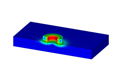
Non-destructive Testing/ Evaluation
EMWorks provides electromagnetic simulation tools to design and assess NDT/NDE sensors such as eddy-current and probe-based systems. Predict signals, coverage, and defect sensitivity before physical testing.
Passive components
Use EMWorks to simulate RF and microwave passive components directly on 3D geometry. Evaluate S-parameters, impedance, loss, and field distribution so you can tune filters, couplers, power dividers, terminations, and interconnects before fabrication.
Permanent Magnets
Use EMWorks to model permanent magnets and magnet arrays—inside motors, actuators, sensors, and couplers. Compute fields, forces, torque, and demagnetization so you can refine geometry and materials before prototyping.
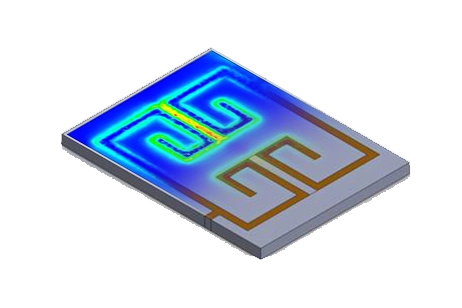
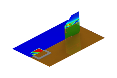
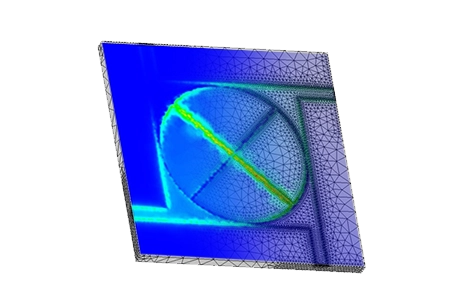
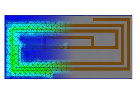
Planar-Printed Antennas
Use EMWorks to model microstrip, patch, and other planar printed antennas on your PCB or package layout. Evaluate impedance match, gain, radiation pattern, bandwidth, and coupling before fabrication.
.webp)
Printed Circuit Boards (PCBs)
Use EMWorks to simulate real PCB layouts, including traces, vias, planes and components. Evaluate signal and power integrity, EMI, and heating so you can fix issues and optimize stackups before fabrication.
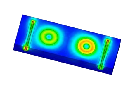
Resonators
Use EMWorks to design RF and microwave resonators, extracting resonant modes, unloaded Q, and coupling for cavity, dielectric, and planar structures.
Sensors
EMWorks provides electromagnetic simulation tools to design and validate sensors for position, current, pressure, and NDT/NDE applications. Evaluate sensitivity, range, and interference before building hardware.
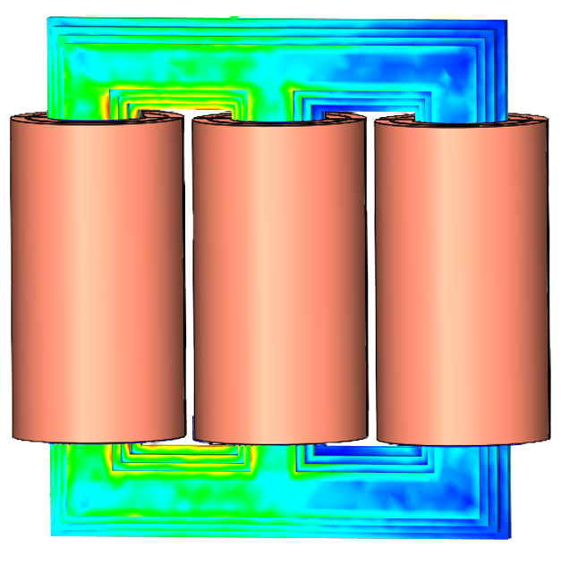
Transformers
Use EMWorks transformer simulation to evaluate core losses, leakage, insulation stress, and temperature rise for power, distribution, and instrument transformers directly from CAD models.
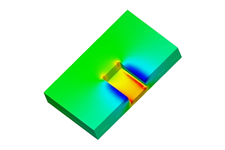
Transmission Line
Simulate RF and microwave transmission lines to predict impedance, loss, dispersion, and crosstalk so you can tune geometry and materials and validate performance before fabrication.
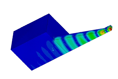
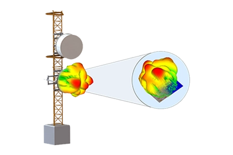
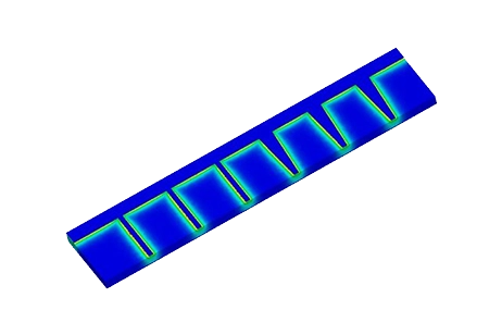
Waveguide Antennas
Use EMWorks to model horn, slotted, and array waveguide antennas on full 3D geometry. Evaluate impedance match, gain, beam pattern, side-lobes, and bandwidth before building hardware.
Wire Antennas
Use EMWorks to model dipole, monopole, loop, helical, and custom wire antennas on full 3D geometry. Evaluate impedance match, gain, radiation pattern, bandwidth, and coupling to nearby structures before you build hardware.
.webp)
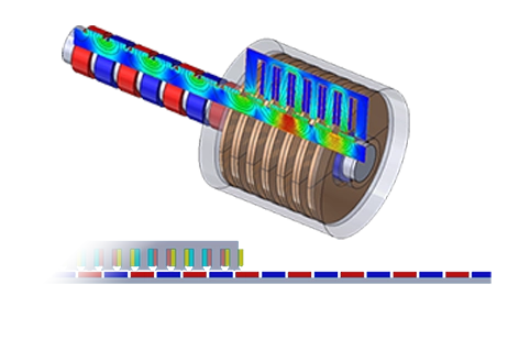
Wireless Power Transfer
Simulate wireless power transfer coils, fields, and coupling directly from your CAD models. Evaluate efficiency, losses, misalignment, and shielding before building prototypes.