Induction Heating
Induction heating is a precise, rapid, consistent, and energy-efficient method for heating electrically conductive materials, including metals. This technique involves applying a high-frequency alternating current to an induction coil, producing a time-varying magnetic field. The material requiring heating is positioned within this magnetic field, without direct contact with the coil. Consequently, the alternating electromagnetic field induces eddy currents within the workpiece, resulting in resistive losses that ultimately translate into heat within the workpiece. Notably, ferrous metals respond particularly well to induction heating due to the heat generated by hysteresis loss. Figure 1 illustrates a typical induction heating configuration.
In this instance, we will demonstrate how to employ EMS in conjunction with thermal analysis to simulate the hardening process of a spherical object placed inside a coil.

Figure 1 - Induction heating setup
Electromagnetic-Thermal coupling capability of EMS
EMS provides the capability for multi-physics simulations, allowing for the seamless integration of electromagnetic, structural, and thermal fields. In our specific scenario, we conducted an electromagnetic-thermal simulation. To address the induction heating challenge within a time-varying domain, EMS necessitates the utilization of a transient magnetic study coupled with thermal analysis.
Problem description
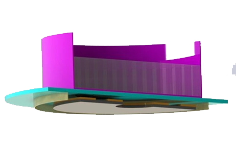
In this demonstration, we will illustrate the induction heating phenomenon as it applies to a sphere enclosed within a coil. Figure 3 displays a 3D CAD representation of the simulated model. The excitation waveform follows a sinusoidal pattern with a frequency of 60 Hz.
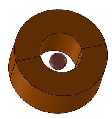
Figure 3 - The simulated model
Simulation setup
Upon establishing a Transient Magnetic study coupled with thermal analysis in EMS, it's essential to adhere to these four crucial steps:
-
apply the proper material for all solid bodies
-
apply the necessary electromagnetic inputs
-
apply the necessary thermal inputs
-
mesh the entire model and run the solver
Materials
Both coil and sphere are made of copper.
Table 1 - Material properties
| Components / Bodies | Relative Permeability | Electrical Conductivity | Thermal Conductivity (W/m*K) | Specific Heat (J/Kg*K) | Masse Density (Kg/m^3) |
| Sphere/ Coil | 1 | 5.840e+7 | 401 | 384 | 8960 |
Electromagnetic inputs
In this study, only a wound coil is assigned as electromagnetic input.
| Number of turns | RMS total current | |
| Wound coil | 1000 | 6.468 A |
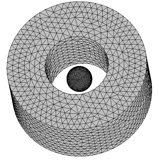
Meshing
Meshing plays a pivotal role in every Finite Element Analysis (FEA) simulation. EMS employs a comprehensive approach to estimate an appropriate global element size for the model, taking into account its volume, surface area, and various geometric intricacies. The actual size of the resulting mesh, including the number of nodes and elements, is contingent upon several factors, such as the model's geometry, dimensions, specified element size, mesh tolerance, and mesh control.
In the initial stages of design analysis, where approximate results may suffice, opting for a larger element size can expedite the solution process. However, for situations demanding a higher degree of precision, a smaller element size becomes imperative to attain a more accurate solution.
Electromagnetic-thermal results
Once the setup is complete, successful execution of the Transient Magnetic simulation coupled with thermal analysis yields comprehensive transient results encompassing both magnetic and thermal aspects.
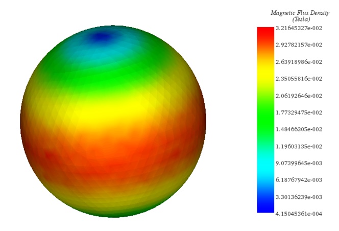
In the following figure, you'll find a 3D plot illustrating the magnetic flux density within the sphere at the 50 ms mark.
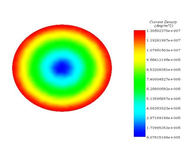
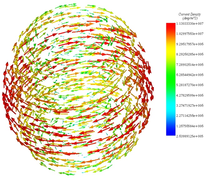
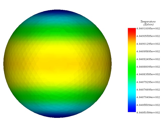
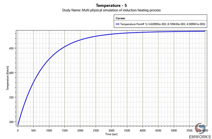
Figures 6 and 7 provide 3D plots illustrating the distribution of current density, depicting the circulation of eddy currents on the surface of the sphere. In Figure 8, you can observe the temperature distribution within the sphere after 1.6 hours.
Conclusion
The application note delves into the intricacies of induction heating, a method prized for its precision, rapidity, consistency, and energy efficiency in heating electrically conductive materials, particularly metals. Through the application of high-frequency alternating current to an induction coil, a time-varying magnetic field is generated, inducing eddy currents within the workpiece, thereby producing heat through resistive losses. The note focuses on employing EMS in tandem with thermal analysis to simulate the hardening process of a spherical object placed within a coil. Demonstrating EMS's electromagnetic-thermal coupling capabilities, the simulation setup involves a transient magnetic study coupled with thermal analysis to accurately model the induction heating phenomenon. The setup encompasses crucial steps including material assignment, electromagnetic inputs, and meshing techniques. Detailed results, including magnetic flux density, current density distribution, and temperature evolution within the sphere, provide insights into the induction heating process. The application note serves as a comprehensive guide for engineers seeking to understand and utilize induction heating through simulation techniques, demonstrating the effectiveness of EMS in multi-physics simulations.