Optimizing Induction Cooking Efficiency through Pot Thickness Analysis

Used Tools:

Induction Cooking

Induction cooking, shown in Figure 1 [1], is gaining popularity worldwide for its efficiency and safety [2], [3]. However, it requires specific ferromagnetic vessels like iron or stainless steel [2]. This method involves passing high-frequency current through a coil under the pan, inducing eddy currents that generate heat via the Joule effect. To enhance efficiency, optimal material properties such as electrical resistivity and permeability are crucial. This study aims to determine the best material properties and thickness for maximizing thermal power.

Figure 1- Induction cooktop installed in a home kitchen [1]

Figure 2 - Induction cooker principle [4]

Problem description

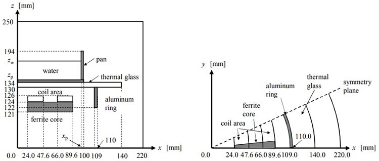
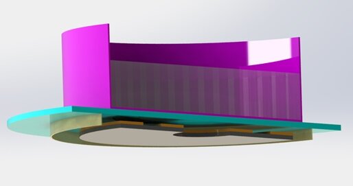
This article focuses on simulating an induction cooker using EMS for a coupled electro-thermal analysis. It will compute eddy losses, winding losses, and temperature predictions. The simulated system includes a pan with water, an aluminum ring, a ferrite core, and glass thermal insulation [5]. Figure 3 illustrates the model geometry, while Figure 4 shows the 3D CAD model. The dimensions are x = 98.5 mm, y = 135.5 mm, and z = 168.3 mm. Two copper wound coils with 10 turns each conduct 24A rms at a frequency of 23.4 kHz.

Geometrical parameters of the simulated model

Figure 3 - Geometrical parameters of the simulated model [6]

Figure 4 - Cross-section view of the simulated CAD model

Optimization of an induction cooker pot

EMS's AC Magnetic module addresses induction cooking challenges, handling linear and nonlinear electromagnetic equations in the frequency domain. It seamlessly integrates with thermal, structural, and motion analyses, making it ideal for tasks like examining eddy current problems, wireless power transfer, and NDT applications.

In the first phase, the module computed eddy losses in the pan due to induced currents from varying magnetic flux. Different material properties were explored. Next, thermal analysis compared temperature changes in two materials, coupled with transient thermal analysis. Finally, varying the pan bottom thickness allowed for plotting the relationship between thickness and eddy loss, utilizing parameterized AC Magnetic simulations.

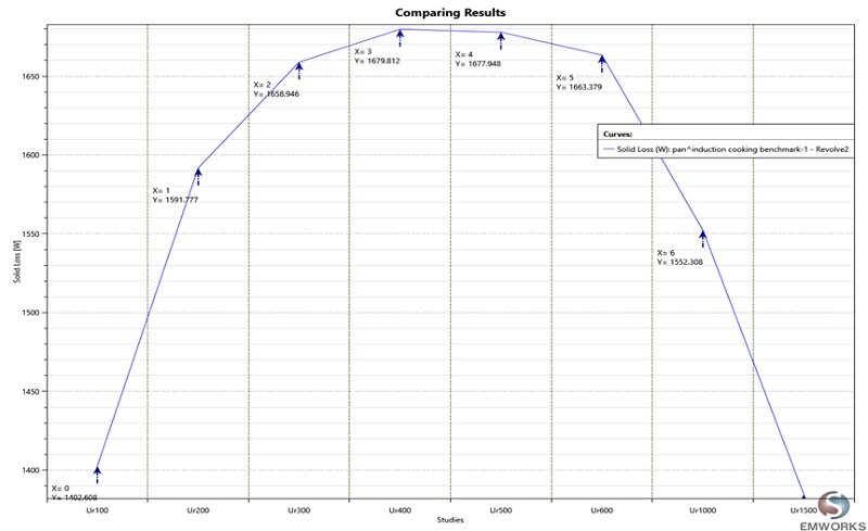
Scenario 1 involves varying the relative permeability while keeping the electrical resistivity constant at $rho égal à 9.7 calligraphique e puissance moins 7 fin de l'exposant omega majuscule calligraphique m espace$ . The relative permeability ranges from 100 to 1500. EMS computes the eddy losses for each case, depicted in Figure 5. The thermal loss (eddy loss) increases with the relative permeability until reaching a peak at $mu indice r égal à 400 espace$ , after which it decreases, as illustrated in the figure.

Eddy loss plot versus relative permeability

Figure 5 - Eddy loss plot versus relative permeability

Scenario 2: Varying the electrical resistivity and keeping the relative permeability constant
In this scenario, the relative permeability is maintained invariably at the value of $mu indice r égal à 400 espace$ while the electrical resistivity is varied from $rho égal à 1 calligraphique e puissance moins 5 fin de l'exposant omega majuscule calligraphique m espace$ to $rho égal à 2 calligraphique e puissance moins 7 fin de l'exposant omega majuscule calligraphique m espace$ .The thermal power versus the electrical resistivity is shown in Figure 6. The eddy loss increases from 1.5 kW at $rho égal à 1 calligraphique e puissance moins 5 fin de l'exposant omega majuscule calligraphique m espace$ to reach 1.8kW at $rho égal à 2 calligraphique e puissance moins 5 fin de l'exposant omega majuscule calligraphique m espace$ , then it decreases to 1.1kW at $rho égal à 2 calligraphique e puissance moins 7 fin de l'exposant omega majuscule calligraphique m espace$ .

Eddy loss versus electrical resistivity

Figure 6 - Eddy loss versus electrical resistivity

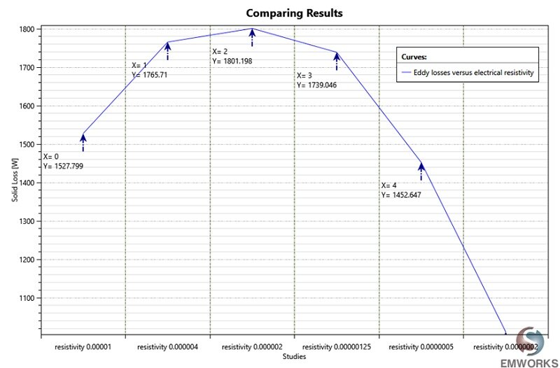
From the previous analyses, a generic material with an electrical resistivity of $rho égal à 2 calligraphique e puissance moins 6 fin de l'exposant omega majuscule calligraphique m espace$ and a relative permeability of $mu indice r égal à 400 espace$ gives an optimal thermal power which is about 1.8kW .

Electromagnetic thermal analysis of an induction cooker with different pot materials:
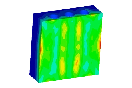
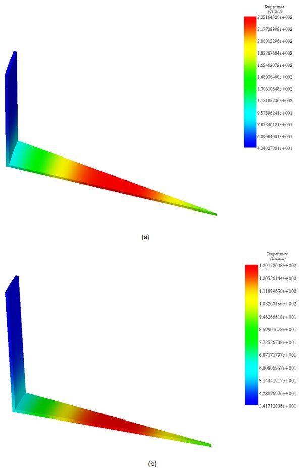
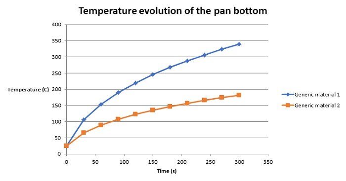
Two generic materials are selected based on prior analyses to examine the impact of eddy losses on temperature evolution. The AC Magnetic module, coupled with transient thermal analysis, is utilized for this investigation. Table 1 summarizes the properties and thermal power of each material. Due to rotational symmetry, only a small portion (1/48) of the model is simulated to save computation time. Figures 7(a) and 7(b) show the temperature distribution of the pan after 2 minutes, while Figure 8 illustrates the temperature rise over time for each pan. Material 1 heats faster and to a higher temperature than Material 2 due to its higher resistivity and lower permeability.

	Generic material 1	Generic material 2
Relative permeability	400	1500
Electrical resistivity	2e-6 $omega majuscule calligraphique m espace$	9.7e-7 $omega majuscule calligraphique m espace$
Thermal conductivity	80	80
Specific Heat	444	444
Mass Density	7860	7860
Generated thermal power	1801.198 W	1384.8 W

Figure7 - Temperature of the pot after 120s : (a)Generic material 1, (b) Generic material 2

Figure 8 - Temperature evolution of the pan bottom versus time

Figure 9 - Temperature rising of the pan made of generic material 1 and the water

Electromagnetic thermal analysis of an induction cooker with varying pot thickness:

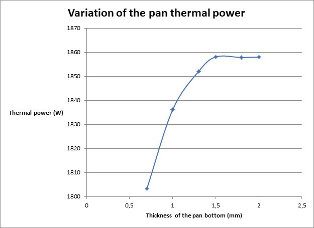
EMS facilitates optimization analysis through parameterized study, enabling the adjustment of both geometric and simulation parameters. In this instance, the bottom thickness of the pot is varied. Eddy loss at each thickness is plotted in Figure 10. The graph indicates that eddy loss in the pot increases from 1 mm thickness and stabilizes around 1.5 mm, primarily due to the skin effect phenomenon. Figure 11 provides an animation depicting the eddy loss density versus pan thickness.

Variation of the pan thermal power versus the thickness of its bottom

Figure 10 - Variation of the pan thermal power versus the thickness of its bottom

Figure 11 - Animation of the eddy loss density versus the pan thickness

Conclusion

The results obtained from the analysis of the eddy loss density versus pan thickness provide valuable insights into the behavior of the induction cooking system. By varying the thickness of the pot bottom, we observe how the distribution of eddy losses changes, influencing the overall thermal performance of the system.

As depicted in the animation, the eddy loss density initially increases as the thickness of the pot bottom decreases from 1.5 mm. This trend is expected due to the skin effect phenomenon, where the induced currents are concentrated in a thin surface layer of the pot. Consequently, reducing the thickness of the pot bottom leads to a higher density of eddy losses, as more of the material is subjected to the influence of the magnetic field.

However, beyond a certain threshold, around 1.5 mm in this case, the eddy loss density stabilizes, indicating a diminishing return in terms of increasing thickness. This phenomenon can be attributed to the saturation of the skin effect, where further reductions in thickness have minimal impact on the distribution of induced currents and, consequently, the density of eddy losses.

These findings have significant implications for the design and optimization of induction cooking systems. Designers can use this information to determine the optimal thickness of the pot bottom, balancing the need for efficient heat generation with considerations such as material cost and structural integrity. Additionally, these results highlight the importance of leveraging simulation tools like EMWorks to gain deeper insights into system behavior and inform design decisions effectively.

References

[1]:https://www.consumerreports.org/electric-induction-ranges/pros-and-cons-of-induction-cooktops-and-ranges/
[2]:https://www.nytimes.com/2010/04/07/dining/07induction.html
[3]:http://www.nicecook.in/facts-about-induction-cookers/induction-cooker-pros-and-cons
[4]:http://garnisoldanella.com/induction-cooktop-frequency/induction-cooktop-frequency-how-does-an-induction-cooktop-work-its-cooking-mechanism-4-burner-gas-cooktop/
[5]:Li Qiu, XiboWen, Hongshen Liand Tiegang Li.Study on effect of material property on thermal power in induction cooker system with finite element method. International Journal of Applied Electromagnetics and Mechanics, vol. 46, no. 1, pp. 35-42, 2014
[6]:DaigoYonetsu and Yasushi Yamamoto. Estimation Method for Heating Efficiency of Induction Heating Cooker by Finite Element Analysis.The Journal of the Institute of Electrical Installation Engineers of Japan,2014 Volume 34 Issue 5 Pages 339-345

Share on