Magnetic Gears
Magnetic gears, favored for their contactless transmission, address the shortcomings of traditional gears such as friction, maintenance needs, and noise. They enhance efficiency and reliability in various industries, including automotive and marine. This article focuses on a coaxial magnetic gear system, analyzed with 2D and 3D simulations to validate its performance and design advantages using the finite element method.
2D FEM simulation of coaxial magnetic gear [2]
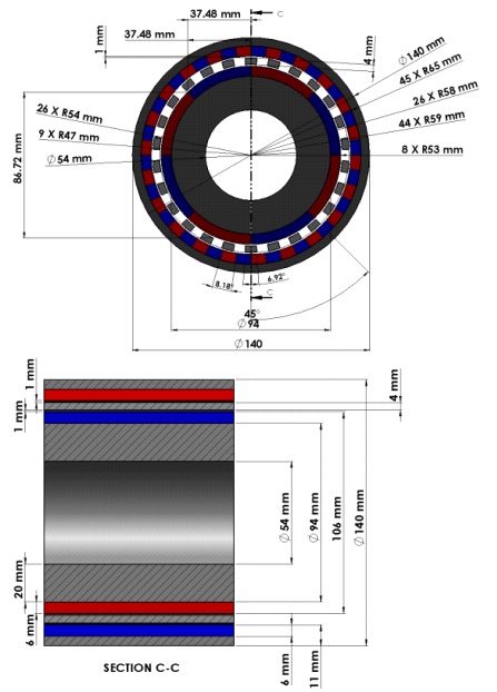
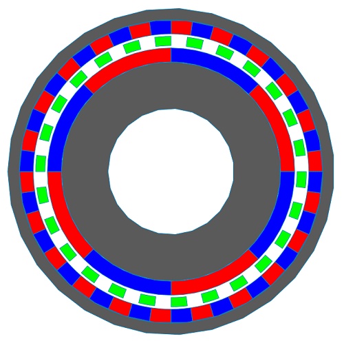
A coaxial magnetic gear model is presented in [2]. The proposed MG is made of 4 pole pairs in the inner rotor, 22 pole pairs in the outer rotor, and 26 modulating pole pieces. So, the model has a gear ratio of $$ G_r = \frac{22}{4} = 5.5 $$.
In the magnetic gear system, the inner rotor rotates faster than the outer rotor, yet it's the slower-moving outer rotor that produces more torque. This phenomenon is analyzed with EMWorks2D, focusing on the magnetic flux within the air gap and the torque generated, while ignoring eddy and end effects for simplicity. Figure 2 provides a visual representation of the magnetic gear's design and dimensions.
The model is displayed in Figure 3. The inner rotor is rotating with the speed of $$ \theta_i = 150 $$ rpm while the speed of the outer rotor is $$ \theta_o = \frac{\theta_i}{G_r} = \frac{150}{5.5} \approx 27.27 $$ rpm. The rotor cores and the modulator are made of steel 1008 characterized by the BH curve demonstrated in Figure 4. NdFeB 35 permanent magnets are used and their properties are presented in Table 1.
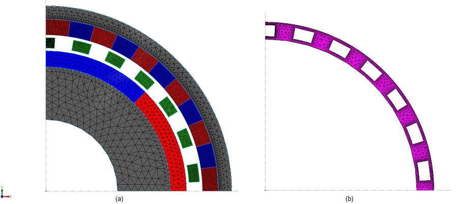
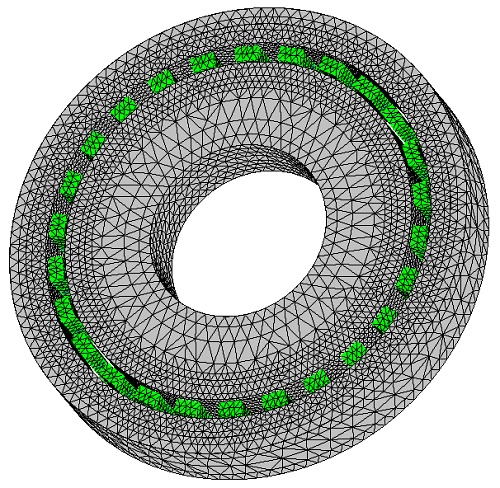
In a parametric Magnetostatic simulation using EMWorks2D, the angles of the inner and outer rotors are variably set. This process is depicted in Figures 3a) and 3b), where the model's mesh and the air gap are highlighted. EMWorks2D automatically generates triangular mesh elements and offers the flexibility to specify mesh element sizes for targeted surface areas or edges, enhancing simulation accuracy and efficiency.
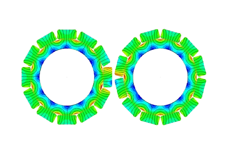
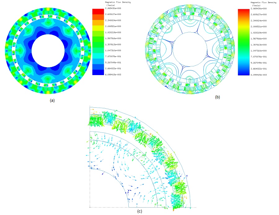
During the simulation, the angles of the inner and outer rotor are linked by the following equation: $$ \theta_o = - \frac{\theta_i}{G_r} $$ . Fringe, vector and line plots of the magnetic flux density are exhibited in Figures 4a), 4b) and 4c) ( $$ \theta_o = 0 \, \text{deg} $$ and $$ \theta_i = 0^\circ $$), respectively. The magnetic field plots are characterized by high flux spots in the ferromagnetic pieces.
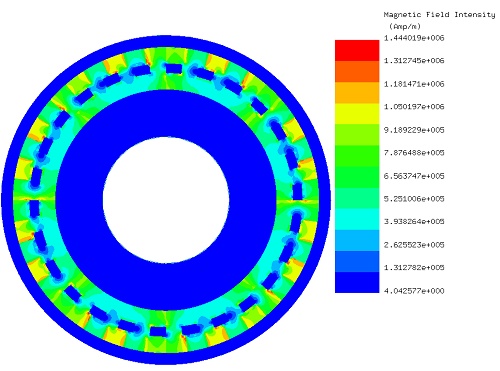
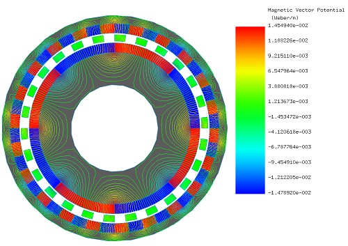
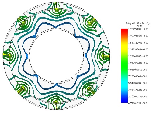
Field lines and vector plots are instrumental in identifying and verifying the directions of flux. Figures 5 and 6 depict, respectively, the fringe plot of magnetic field intensity and the contour lines plot of magnetic vector potential, offering visual insights into the magnetic flux patterns within the system.
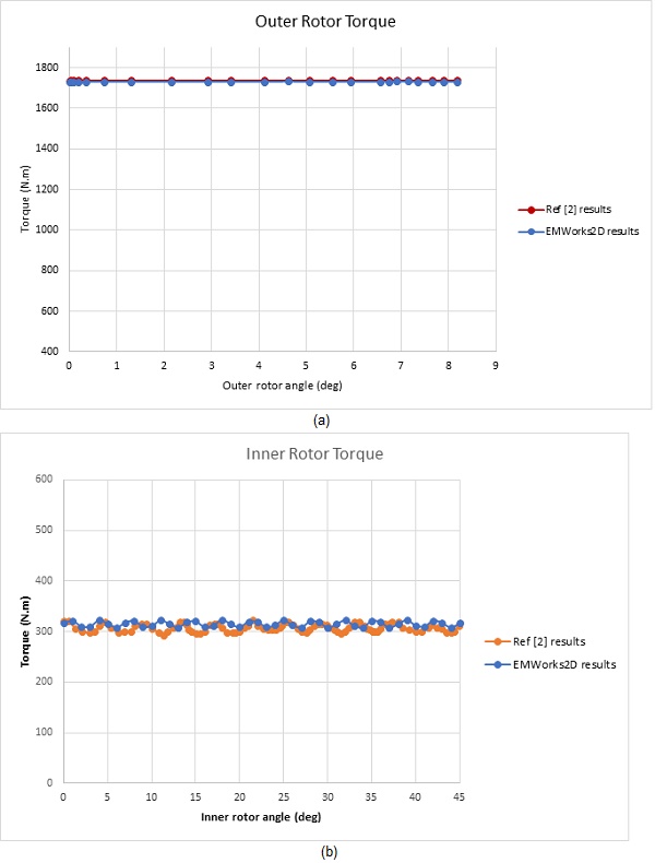
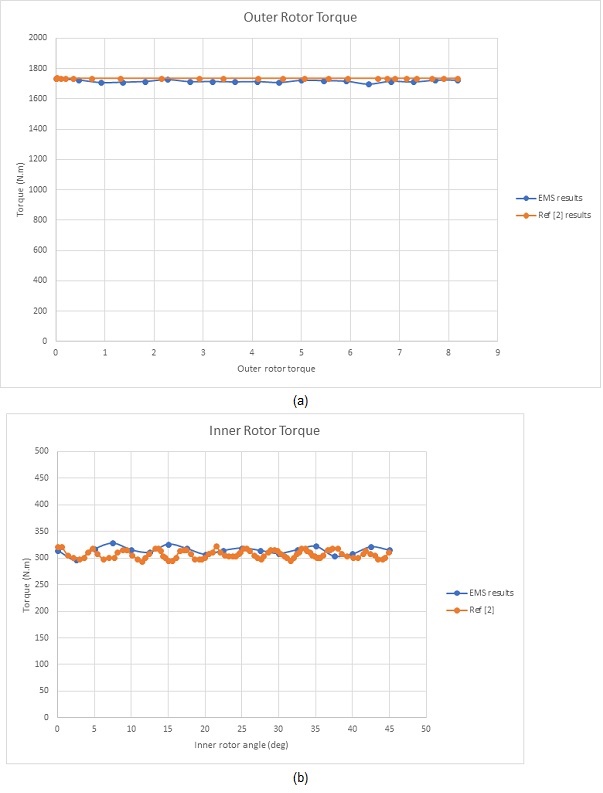
Figures 7a) and 7b) showcase the torque generated in the outer and inner rotors, respectively. Consistent with earlier observations, the slower-moving outer rotor generates a higher torque compared to the faster inner rotor. The outer rotor's design, featuring a higher number of pole pairs, results in smoother torque fluctuations as seen in Figure 7a), in contrast to the more pronounced ripples in Figure 7b)'s torque curve. Initially, the torque reaches approximately 1737 N.m in the outer rotor and about 315 N.m in the inner rotor, thereby confirming the gear ratio relationship between the two rotors.
3D FEM simulation of the coaxial magnetic gear
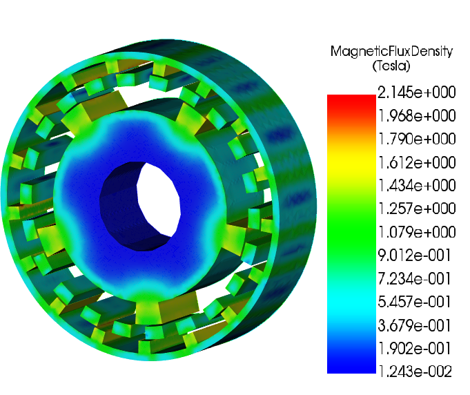
The magnetic gear model initially explored with EMWorks2D is revisited for analysis through EMS, a 3D electromagnetic simulation software, while retaining the original dimensions. Due to the axial symmetry of the model, simulating a partial segment is recommended to enhance efficiency. Thus, a 20 mm section of the gear is analyzed instead of the entire 300 mm length, significantly reducing computational demands. Figure 8 illustrates the 3D model of the geometry being examined.
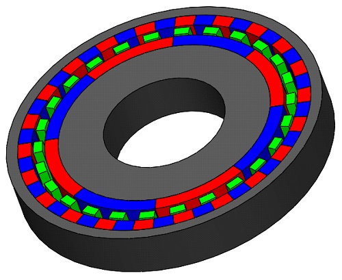
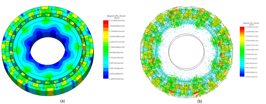
Figure 8 illustrates the model, meticulously meshed with tetrahedral elements known for delivering precise solutions. The magnetic flux density is visually analyzed in Figures 9a) for fringe plots and 9b) for vector plots, highlighting the flux patterns.
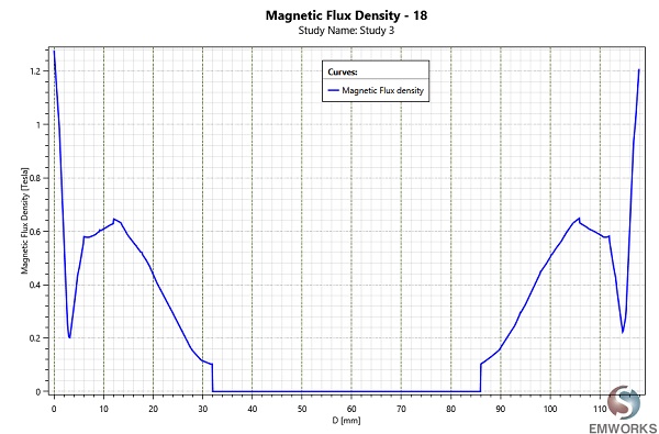
Iso surfaces of magnetic flux density within the inner rotor are depicted in Figure 10, offering a detailed view of magnetic interactions. Figure 11 presents a magnetic field plot along a line between two poles of the outer rotor. This plot features a symmetrical shape around the model's midpoint, indicating that analyzing just one-half of the curve suffices. At the magnet's surface on the outer rotor, the field reaches its maximum, then decreases through the air gap, and increases again, forming two peaks in the inner rotor's magnet region, before finally tapering off near zero in the shaft area, simulated as air in this study.
Figures 12a) and 12b) detail the torque outcomes for the outer and inner rotors, aligning with the 2D EMWorks2D simulations. The outer rotor, moving at a lower speed, generates a torque of approximately 1730 N.m, while the faster inner rotor achieves around 310 N.m.
The comparison of data in Figures 7 and 12 confirms the consistency between 2D and 3D simulation results, validating the effectiveness of both EMWorks2D and EMS 3D FEM software in predicting magnetic gear performance. Moreover, Figure 13 showcases an animated plot of magnetic flux density against the rotation angles of both rotors, highlighting their opposite rotational directions. This synchronization between 2D and 3D simulations enhances confidence in the accuracy of the modeling techniques used.
Conclusion
This application note delves into the analysis of coaxial magnetic gears using 2D and 3D electromagnetic simulations, highlighting their advantages over traditional gears such as maintenance-free operation, absence of friction, and silent functioning. Focused on a coaxial magnetic gear with a gear ratio of 5.5, the study utilizes EMWorks2D and EMS software to assess magnetic flux and torque generation, ignoring eddy and end effects for simplification. The simulations demonstrate the gear's capability to transmit torque without physical contact, with the outer rotor generating more torque at a slower speed due to its design and the number of pole pairs. The findings underscore the magnetic gears' potential across various sectors, particularly automotive and marine, where efficiency and reliability are crucial. Consistent results from both 2D and 3D simulations validate the gear's design and operational efficacy, suggesting magnetic gears as a viable alternative for industries seeking durable and efficient power transmission solutions.
References
[1]: Yawei Wang, Mattia Filippini, Nicola Bianchi, Piergiorgio Alotto. A Review on Magnetic Gears: Topologies, Computational Models and Design Aspects. Published in: 2018 XIII International Conference on Electrical Machines (ICEM), IEEE
[2]: Valentin Mateev, Iliana Marinova and Miglenna Todorova Department of Electrical Apparatus Technical University of Sofia, Bulgaria. Eddy current losses in permanent magnets of a coaxial magnetic gear. Published in: 2018 20th International Symposium on Electrical Apparatus and Technologies (SIELA), IEEE