Introduction
Non-Destructive Testing (NDT) is a process for inspecting materials, components, or assemblies without rendering them unusable. It plays a critical role in ensuring product quality and safety. One valuable electromagnetic NDT method is Alternating Current Field Measurement (ACFM), which we explore in this article using EMS, a 3D field simulation software for designing and testing NDT probes.
What is ACFM?
ACFM (Alternating Current Field Measurement) is a non-destructive electromagnetic technique used to detect and size surface cracks in both ferrous and non-ferrous metals. It offers advantages like minimal surface cleaning, no frequent calibration, and quantitative evaluation. ACFM probes induce eddy currents on the material's surface, creating a magnetic field. When a crack is present, it disrupts these currents and the magnetic field, allowing for crack detection and sizing.
Designing effective ACFM probes involves optimizing parameters like coil size, location, current, and frequency. Experimentation is time-consuming and costly. EMS software, using the Finite Element Method (FEM), simplifies NDT probe design and optimization.
Example of a Twin Coil Inducer ACFM probe [1]
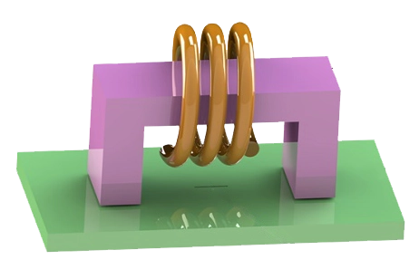
The ACFM probe (Figure 1) includes two coils and an enclosed magnetic sensor within a plastic container. The magnetic sensor detects the magnetic flux density when the probe contacts the test surface and is scanned in the indicated direction. Specifically, it measures the magnetic flux density in the Y direction (By). In the absence of a crack, By remains relatively uniform, but the presence of a surface crack leads to changes in its value. These changes are detected and compared to predefined values to determine the crack size.
Each coil consists of 36 turns of 0.5 mm diameter copper wire, with an RMS current value of 0.6 amps and a frequency of 6 KHz.
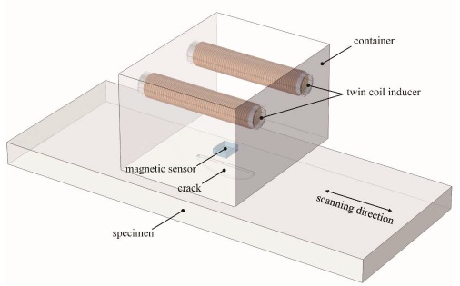
Figure 1 - A model of an ACFM probe [1]
Results from EMS
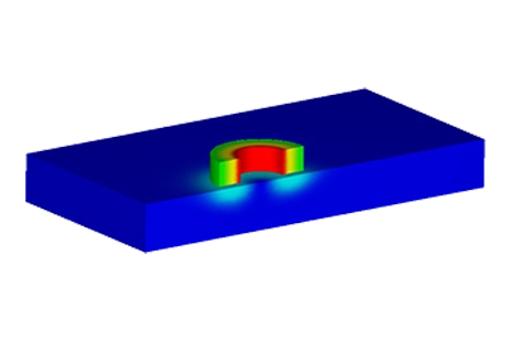
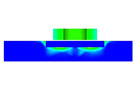
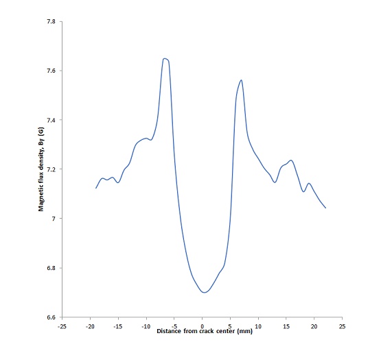
The results from EMS are illustrated in the following figures. Figure 2 displays the distribution of the current density vectors on the specimen, while Figure 3 presents the magnetic flux density (By) on the specimen's surface. Additionally, Figure 4 depicts the changes in magnetic flux density (By) at the magnetic sensor's position as the probe is moved along the length of the crack.
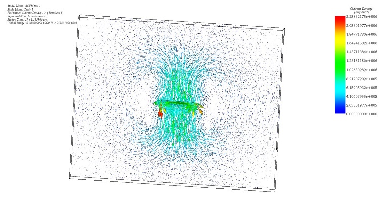
Figure 2 - Current density distribution around the crack
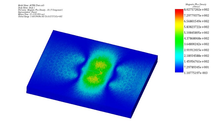
Figure 3 - By distribution on the plate
Figure 3-A - Magnetic Flux Density plot
Conclusion
This application note delves into the use of Alternating Current Field Measurement (ACFM), a non-destructive electromagnetic testing method, for detecting surface cracks in materials using EMS software. ACFM is distinguished by its minimal surface preparation requirements, lack of frequent calibration needs, and its ability to provide quantitative evaluations of crack size in both ferrous and non-ferrous metals. The article showcases the design and simulation of an ACFM probe, including twin coils and a magnetic sensor housed within a plastic container, to optimize parameters such as coil size, location, and current frequency using the Finite Element Method (FEM) for efficient NDT probe creation. Results from EMS simulations illustrate how the probe detects changes in magnetic flux density (By) caused by surface cracks, with visual representations of current density distribution and By variation around the crack. This study emphasizes the effectiveness of EMS in simplifying the design and optimization of NDT probes, thereby enhancing material inspection processes and product safety.
Reference
[1]: Wenpei ZHENG. China University of Petroleum-Beijing, Beijing, Numerical Simulation in Alternating Current Field Measurement. 19th World Conference on Non-Destructive Testing 2016