What is an eddy current brake?
Eddy currents, resulting from electromagnetic induction, have historically posed challenges due to inefficiency and heat generation. However, engineers have developed solutions like laminated materials and cooling systems to mitigate these issues. Nonetheless, eddy currents also have practical applications, such as metal detectors and induction heating. This article focuses on rotary eddy current brakes (ECB), which offer advantages over traditional braking systems by converting kinetic energy into heat via electromagnetic induction. ECBs, utilizing electromagnets or permanent magnets, generate a static magnetic field inducing currents in a rotating disk, producing a braking torque opposite the motion direction. These contactless brakes provide benefits like wear-free operation, low maintenance, and high efficiency, making them suitable for various applications, including trains, automotive engines, and wind turbines. However, free-wheel magnetic brakes have limitations, such as low torque at low speeds and the need for supplementary friction brakes.
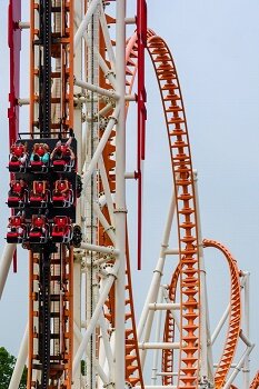
Figure 1 - Roller coaster using eddy current retarder
Simulation of the eddy current brakes (ECB)
Engineers and researchers collaborated to develop innovative eddy current brakes, with finite element (FE) solutions proving reliable for studying magnetic braking [1]. In this study, EMS is used to analyze rotary eddy current brakes, computing parameters like magnetic flux, eddy currents, braking torque, and more.
Two analyses will be conducted:
1. Neglecting transient mechanical response, torque versus time will be computed during constant-speed rotation.
2. Considering transient mechanical response, torque versus time will be computed after applying an initial velocity.
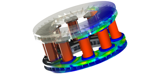
Figures 2a) and 2b) depict the proposed ECB model, comprising a rotating copper disk, permanent magnets, and a back iron core (see Figure 3). The remanence of the permanent magnets is 1.25 T, and the iron core's relative permeability is. $$ \mu_r = 1000 $$ . The electrical conductivity of copper is the following: $$ \sigma = 57 \, \frac{\text{MS}}{\text{m}} $$ while it is neglected for the iron material.
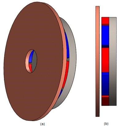
Figure 2 - Eddy current brakes model, a) isometric view b) side view
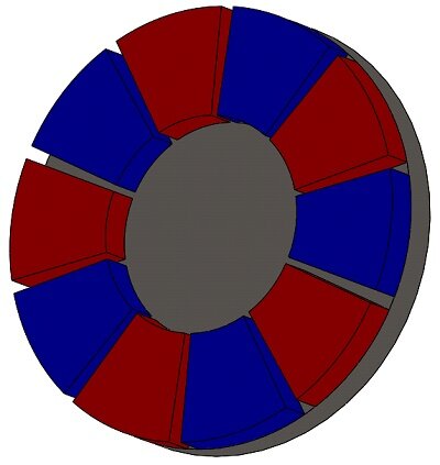
Figure 3 - Arrangement of the permanent magnets and back iron core
In Figure 4, a cross-sectional view of the mesh plot is depicted, showcasing element sizes ranging from 1.3 mm in the copper disk to 10 mm in the iron core. The mesh can be customized manually using the EMS mesher, with smaller element sizes applied on the disk surfaces to effectively capture eddy currents.
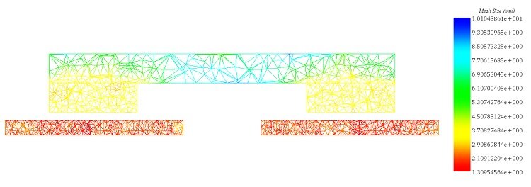
Figure 4 - Cross-section view plot of the mesh
Results and Discussions
Constant Speed
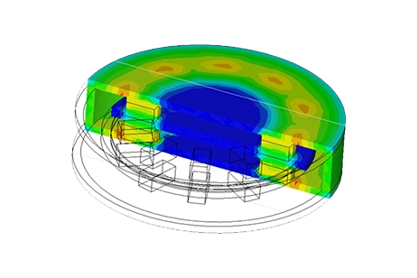
In this setup, the copper disk rotates steadily at 1000 rpm in the counterclockwise direction, inducing eddy currents within it. These currents generate an opposing electromagnetic torque. Figures 5a) and 5b) depict fringe and vector plots of the magnetic flux density in the permanent magnets and iron core, respectively. The magnets alternate in direction along the iron core axis, while the iron core reduces magnetic flux losses and aligns the field with the disk's direction. It also acts as a magnetic shield, protecting electronics like rail sensors and signals from electromagnetic interference. Figure 6 shows the H field plot.
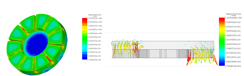
Figure 5 - Magnetic flux density, a) fringe plot, b) vector plot (cross-section view)
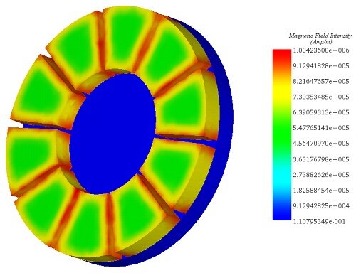
Figure 6 - Magnetic field intensity
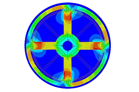
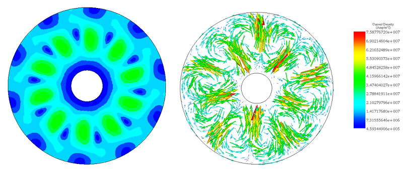
The figures display the distribution of eddy currents within the copper disk, with multiple loops aligning with each magnet pole's direction. The highest induced current reaches 1.6e7 A/m². Due to the constant speed, eddy currents remain unchanged over time, as shown in the animation in Figure 8.
 (a) (b)
 Figure 7 - Eddy currents, a) fringe plot b) vector plot
Figure 8 - Animation of the current distribution
Figure 9 displays torque results at speeds of 500 and 1000 rpm. In both cases, torque remains constant and negative over time, opposing the disk's rotation according to Lenz's law. The blue curve represents torque at 500 rpm, while the red curve depicts torque at 1000 rpm. Notably, the blue curve shows lower torque values (10 Nm) compared to the red curve (12.6 Nm), indicating that higher speeds result in higher torque. This underscores the suitability of such brakes for high-speed applications. However, increased speed may lead to higher heat generation in moving parts.
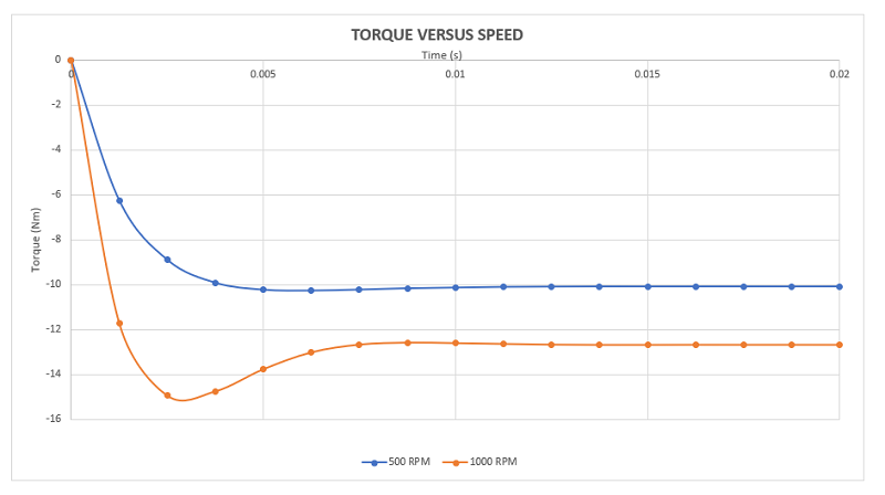
Figure 9 - Generated torque for different speed rate
Braking phase
This section focuses on decelerating the disk from its initial rotation at 1000 rpm using braking torque while suppressing load torque. EMS's Transient Module, combined with Motion analysis, handles both electromagnetic and mechanical aspects during the 0.2-second transient simulation.
Figure 7 illustrates the evolution of eddy currents as the disk rotates within the static magnetic field generated by the permanent magnets. At 0.005s (Figure 7a), a peak current density of approximately 6.4e+7 A/m² occurs at a velocity of 1000 rpm. As the speed decreases to 135 rpm (0.05s), the maximum eddy current density drops to about 1.75e+7 A/m². By 0.17s, with the speed reduced to 0.35 rpm, the average current density notably diminishes.
This trend highlights the direct relationship between eddy currents and speed, with the presence of eddy current loops diminishing as speed approaches zero.
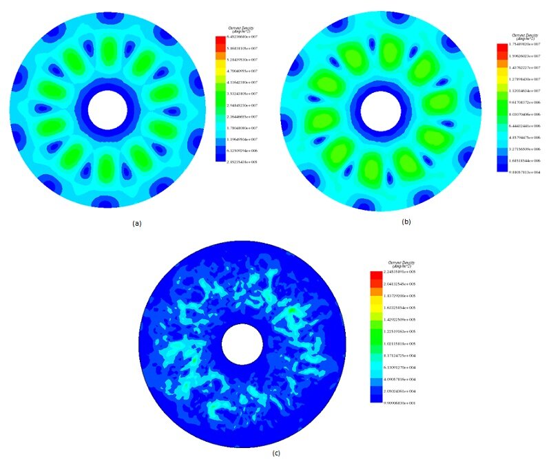
Figure 10 - Eddy current distribution, a) at 0.005s b) at 0.05 c) at 0.17s
Figure 11 illustrates the eddy losses (W) resulting from the eddy currents within the spinning disk. Mirroring the current density trend, it peaks at 900W at 0.005s when the speed reaches its maximum (1000rpm), gradually decreasing as the disk decelerates.
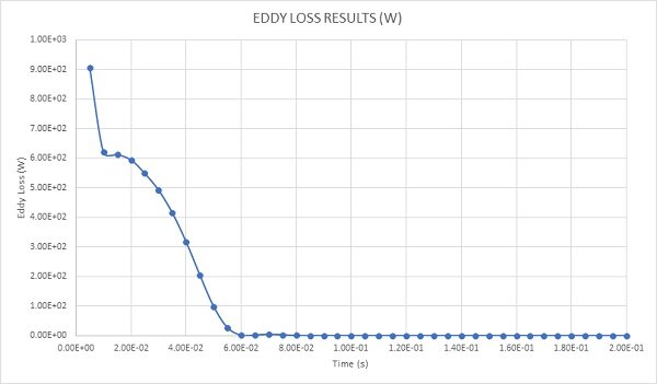
Figure 11 - Eddy loss
Figure 12 depicts the electromagnetic torque curve alongside the angular speed of the disk. Initially, the torque declines from -3.7 Nm at 0.005s to -2.24 Nm at 0.01s before peaking at around -6 Nm at 0.04s. Concurrently, the disk's velocity decreases from its peak of 1000 rpm at 0.005s to zero at 0.057s. Notably, both torque and speed exhibit opposite directions, with the disk rotating anticlockwise while the torque acts clockwise until 0.057s, and vice versa thereafter (Lenz’s law).
As the speed continues to decrease, the torque diminishes accordingly. Upon reaching a steady state at 0.1s, both the electromagnetic torque and speed approaches zero. Remarkably, the magnetic brake achieves complete cessation of disk rotation within 0.057s.
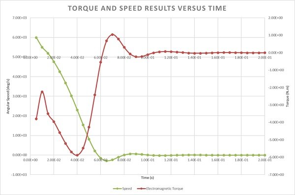
Figure 12 - Braking torque and angular speed curves
Figure 13 compares the angular positions of the disk under two conditions: with and without the influence of eddy currents. The blue curve represents the scenario where no eddy currents are present, allowing the disk to rotate freely. During the simulation period of 0.2s, it completes 3.33 revolutions. Conversely, the red curve depicts the disk's angular displacement when eddy currents are active, leading to the application of braking torque. In this case, the disk comes to a stop at 0.57s after rotating 161 degrees.
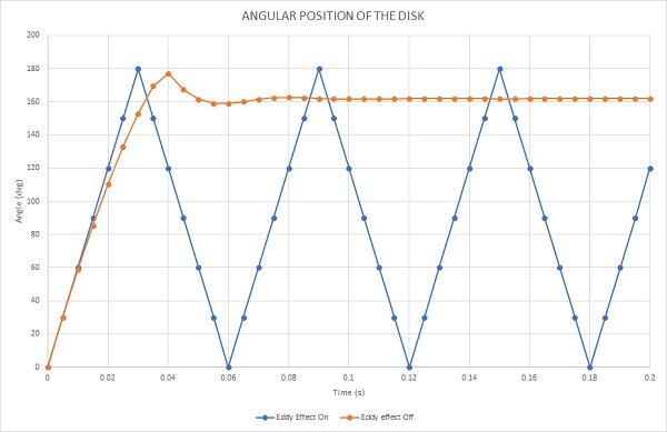
Figure 13 - Angular displacement of the disk
Figure 14 presents an animation depicting the distribution of eddy currents as the disk decelerates. It visually illustrates the reduction in current intensity as the speed decreases..
Figure 14 - Eddy currents versus time during the braking phase
Conclusion
The application note delves into the principles and applications of rotary eddy current brakes (ECB), showcasing their contactless operation that transforms kinetic energy into heat through electromagnetic induction. Unlike conventional brakes, ECBs suffer no wear, require minimal maintenance, and offer efficient braking, making them ideal for trains, automotive engines, and wind turbines. The analysis employs EMS for finite element simulation, focusing on a copper disk, permanent magnets, and an iron core arrangement. The study explores ECB performance under constant and varying speeds, demonstrating how eddy currents induced in the copper disk generate braking torque opposing motion. Results reveal that torque increases with speed, indicating ECBs' suitability for high-speed applications despite potential heat generation concerns. Transient mechanical response simulations further illustrate the braking process, showing a direct relationship between eddy currents and disk speed, with eddy losses peaking at initial high speeds and reducing as the disk decelerates. Ultimately, this study highlights ECBs' effectiveness in providing smooth, efficient braking through electromagnetic principles, offering an advanced solution for automotive applications.
References
[1]: Kerem Karakoc , Afzal Sulemana , Edward J. Park. Analytical modeling of eddy current brakes with the application of time varying magnetic fields. Applied Mathematical Modelling 000 (2015) 1–12