A DC Linear Actuator
Coil heat generation critically impacts the lifespan, efficiency, and repeatability of DC linear actuators. This application note details an electrothermal simulation examining the effects of variables like coil thickness and input currents on heat distribution under various design conditions. It utilizes temperature-dependent material properties to predict actuator temperature changes over time, factoring in the electrical resistivity variations of the coil material.
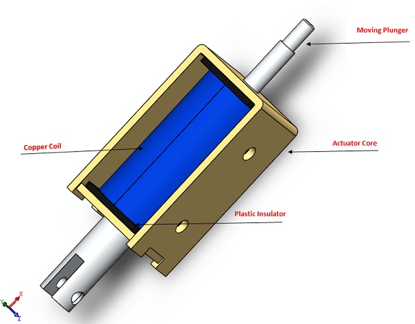
Figures 1 and 2 present the original and simulated 3D CAD models of the actuator, respectively. Non-magnetic components, irrelevant to magnetic outcomes but potentially influencing thermal results, were excluded from this analysis. Additionally, the simulation considers the spring's effect in motion studies when integrated with magnetic analyses.
Figure 2 depicts the simulated DC actuator's components, highlighting the moving plunger and actuator core crafted from 12L14 carbon steel. The coil bobbin, designed for insulation, is made from FEP material.
Simulation & Results
1- Variable Plunger position
In magnetic static simulations, heat generation results exclusively from the Joule Effect within conductors carrying current, making it the sole source of ohmic losses.
The Ohmic loss or winding loss is expressed by the following relation: $$ P = 0.5 \times \rho \times \int J^2 \, dv $$ Where is the electrical resistivity of the coil material and is the current density of the coil.
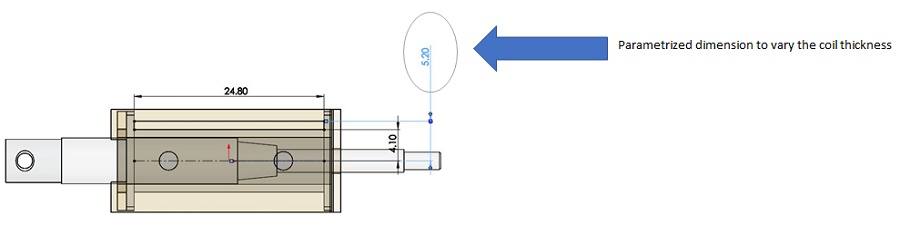
Thus, both Ohmic loss and coil temperature directly correlate with the coil material and current density. With the coil material constant, variations in current density are achieved by altering the coil dimensions. In this analysis, while the input current remains fixed, coil dimensions are adjusted to impact current density, primarily influenced by the coil's cross-sectional area. The key variable under investigation is the coil thickness, as demonstrated in Figure 3.
Figures 4a) and 4b) provide full and cross-section views of the magnetic field distribution for a coil thickness of 2.2mm, the maximum accommodated by the actuator's design. In these configurations, the magnetic field intensity is approximately 0.55T in the actuator core and reaches up to 2T in the moving plunger.
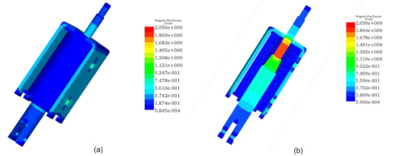
Figures 5a) and 5b) display full and cross-section views of the magnetic field distribution for a coil thickness of 1.1mm, revealing identical magnetic field results to the previous scenario due to the constant input current. Figure 6 provides a vector plot illustrating the magnetic flux distribution.
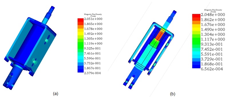
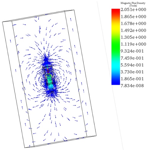
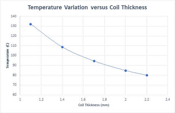
Figure 7 illustrates that current density is inversely proportional to coil thickness, peaking at 1.31e+7 Amp/m^2 with a 1.1mm thickness and dropping to 6.59e+6 Amp/m^2 at 2.2mm. Figure 8 plots Ohmic losses against coil thickness, showing a decrease from 2.65W at 1.1mm to 1.34W at 2.2mm, due to the increase in coil volume with thickness. Temperature trends are expected to mirror these variations.
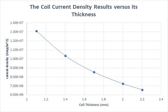
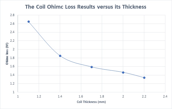
Figure 8 - The coil Ohmic loss versus its thickness
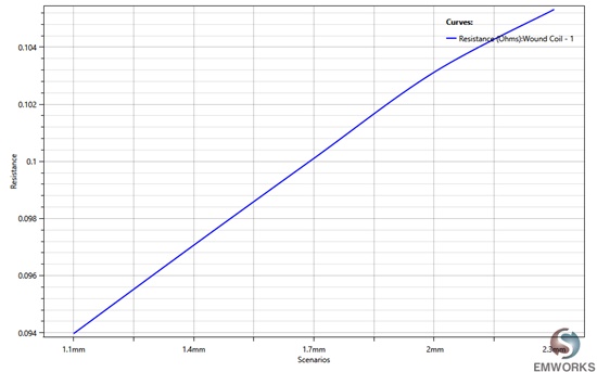
The figure below demonstrates that coil resistance varies linearly with thickness, increasing from 0.094 Ohm at a thickness of 1.1mm to 0.106 Ohm at 2.2mm.
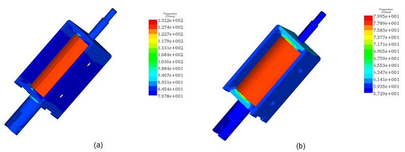
Figures 10a) and 10b) showcase the steady-state temperature distribution within the actuator for coil thicknesses of 1.1mm and 2.2mm, respectively. At a 1.1mm thickness, the temperature reaches 132°C, while at 2.2mm, it reduces to approximately 80°C. The highest temperature is observed at the coil, the primary heat source, with lower temperatures in components in contact with the coil. As the coil thickness increases, heat spreads more extensively throughout the model, as depicted in Figure 10b). Figure 11, displaying temperature variation against coil thickness, mirrors the trend observed in current density variation.
2- Temperature Variation versus Coil current
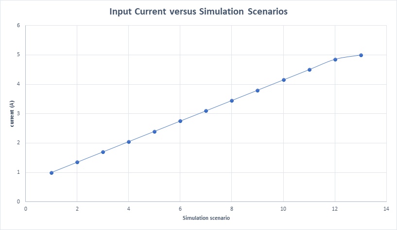
In this analysis, the coil thickness is fixed at 2.2mm while the input current is adjusted, ranging from 1A to 5A in increments of 0.35A for the simulation.
The magnetic flux density results at an input current of 1A, depicted in Figures 13a) and 13b), show a maximum magnetic field of approximately 1.29T in the moving plunger. When the input current increases to 5A, the magnetic field peaks at 2.15T, as illustrated in Figures 14a) and 14b).
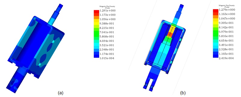
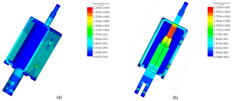
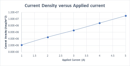
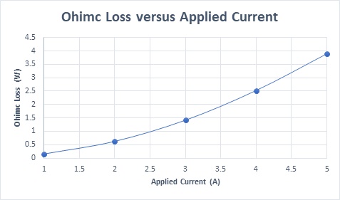
Figure 15 demonstrates the current density results against varying input current rates, showcasing a linear relationship with the input current. Ohmic losses as a function of coil currents are plotted in Figure 16, further illustrating the impact of input current variations on the actuator's performance.
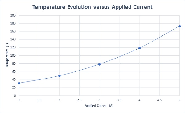
Figures 17a) and 17b) present cross-section plots of the actuator's steady-state temperature at applied currents of 1A and 5A, respectively. At 1A, the actuator's temperature is predicted to range between 30°C and 32°C, whereas at 5A, it escalates significantly, varying from 110°C to 174°C. In both scenarios, the highest temperature is recorded in the coil, from where it disperses throughout the actuator until thermal equilibrium is reached.
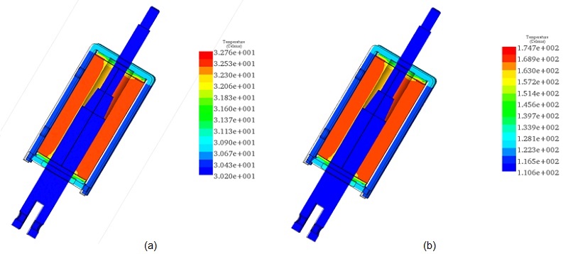
Figure 18 displays the actuator's maximum temperature against various applied current rates, illustrating a temperature increase corresponding to the rise in input current, as previously detailed.
Thermal Analysis in case of temperature-dependent material property
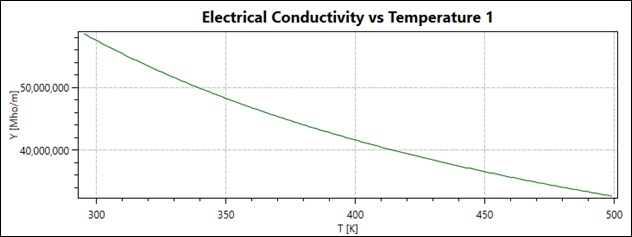
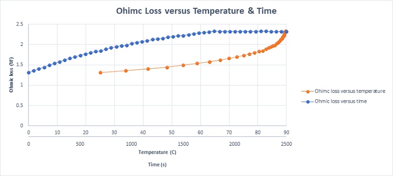
In the concluding section, the copper coil is characterized by temperature-dependent electrical resistivity, highlighting how copper's electrical conductivity decreases as temperature increases—resulting in higher electrical resistivity with rising temperatures. Consequently, as the temperature deviates from ambient, the copper winding's electrical resistivity grows, leading to an increase in Ohmic losses. Figure 20 depicts the coil's Ohmic losses over time and temperature, supporting the notion that copper loss escalates linearly over time, stabilizing at 2.33W after thirty minutes, indicating the attainment of a steady state.
Given the temperature-responsive nature of the coil material, its resistance is similarly impacted. Figure 21 presents a plot of the coil's DC resistance in relation to both time and temperature, demonstrating an increase in resistance with temperature. The resistance starts at 0.1035 Ohm at ambient temperature and reaches a steady state of 0.1295 Ohm after thirty minutes, underscoring the direct relationship between temperature elevation and resistance augmentation in the coil.
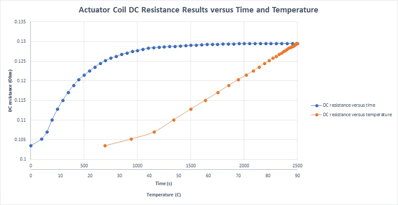
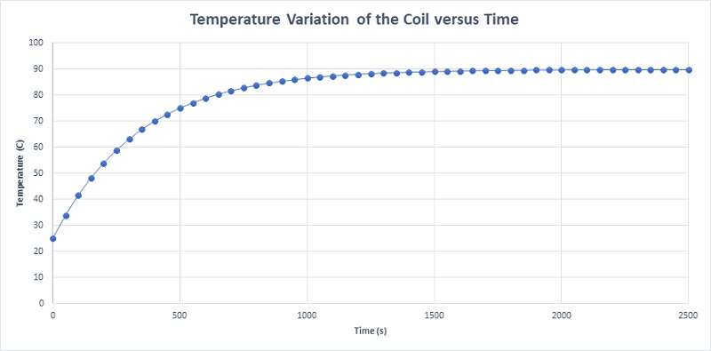
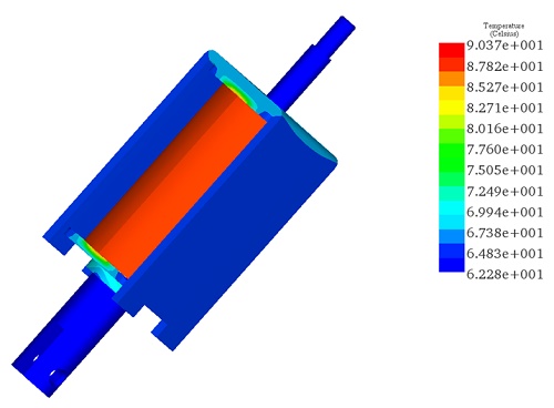
Figure 22 details the temperature variation of the coil, mirroring the progression of Ohmic losses. The temperature escalates from 25°C at the initial moment (t=0) to a steady state temperature of 90.03°C at 1800 seconds (t=1800 s). The steady-state temperature distribution of the actuator, capturing the comprehensive thermal dynamics over time, is plotted in Figure 23.
Conclusion
The electrothermal simulation presented in this application note offers a comprehensive analysis of the heat generation and temperature distribution in a DC linear actuator, crucial for its efficiency and longevity. By examining the impact of variables like coil thickness and input currents on heat distribution, the study provides valuable insights into optimizing the actuator's design for improved performance. Figures and plots depict magnetic field distribution, current density, Ohmic losses, and temperature variations under different conditions, elucidating the intricate relationship between design parameters and thermal dynamics. Key findings include the direct correlation between coil thickness and temperature, as well as the linear relationship between input current and actuator temperature. Additionally, the consideration of temperature-dependent material properties, such as copper's electrical resistivity, highlights the importance of accounting for thermal effects in actuator design. Overall, this analysis offers valuable guidance for engineers and researchers seeking to enhance the reliability, efficiency, and repeatability of DC linear actuators through optimized design and operation strategies.