Magnetic Field on Axis of a Current Loop

Used Tools:

The Biot-Savart law

The Biot-Savart law enables the calculation of the magnetic field created by electric currents. It's a universal law applicable to various current configurations. Essentially, it says that a very small segment of a current-carrying wire generates a magnetic flux density at a certain distance away. This concept is fundamental in understanding how electric currents produce magnetic fields.
The law states that an infinitesimally small current-carrying path produces magnetic flux density  at a distance r:

Where  is the vacuum permeability and  is the unit vector in the direction of the distance. In symmetric problems, it is possible to simplify the analysis and obtain a closed form solution. The field on the axis of a current carrying loop can be easily computed using the Biot-Savart law, due to the fact that only  axis component  of the  vector contributes to the resultant field intensity (Fig. 1):

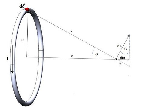
Figure 1- Biot-Savart law and field on centerline of a current loop

The total flux density at a point on the centerline at a distance z is found by integrating the expression for  over the circumference of the loop:

For a current and loop radius , the axial magnetic field is .

Model

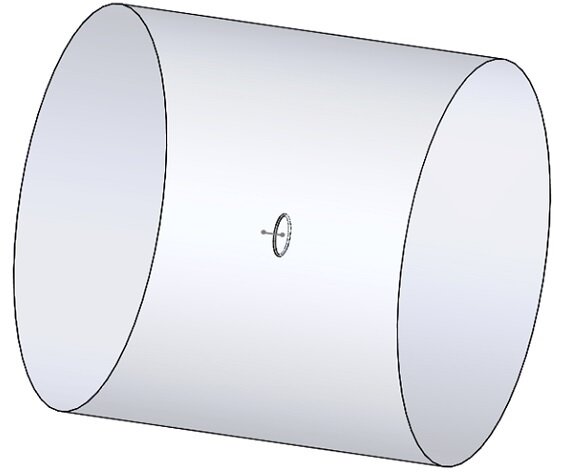
In a simulation using EMS, a thin toroid with a 5mm cross-sectional radius and a 100mm loop radius is modeled in a Magnetostatic study. Copper is used as the material for the toroid, while the remainder of the assembly is air. For precise magnetic field measurements, it's crucial to create a sufficiently large air domain.
For guidance on assigning materials in EMS, refer to the example “Computing capacitance of a multi-material capacitor.” Additionally, the “Electric field inside the cavity of a charged sphere” example provides insights into defining the air domain in EMS.

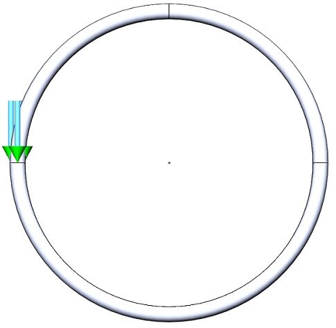
Solid Coil

To apply the EMS Coil feature to the Toroid, access to its cross-sectional surface is needed. Therefore, the procedure involves splitting the Toroid into two separate bodies. This step is essential for the proper application of the feature in the simulation process. For detailed instructions on how to split the Toroid part, you can refer to the source for more comprehensive guidance.

1. Select the Toroid part in the Solidworks feature manager
2. Click Edit component  in the Solidworks Assembly tab
3. In Solidworks menu click Insert/Molds/Split
4. In the Split feature manager, select the Top Plan of the Toroid in the Trim Tools Tab and Click Cut Part
5. In the Resulting Bodies tab, Click Select all.
6. Click OK  

In the EMS feature tree, Right-click on the Coilsfolder, select Solid Coil  .
Click inside the Components or Bodies for Coils box .
Click on the (+) sign in the upper left corner of the graphics area to open the components tree.
Click on the Toroid icon.  It will appear in the Components and Solid Bodies list.
Click inside the Faces for Entry Port box  then select the entry port face.
In the Exit Port Tab, Check “Same as Entry Port“. (Figure 3)

General Properties:

1. Click on General properties tab.
2. Keep default Coil Type as a Current driven coil.
3. Type 100 in the Net current field.
4. Click OK .

Results

To be able to display the variation of the magnetic field along the axis of the Toroid, before running the simulation:

1. In the Assembly, Select the ZX plane and sketch a line going from the center of the toroid along the z axis, with a length of 100mm.
2. Then Insert/Reference geometry/Point and add a Reference point for each end of the line.
3. In the EMS feature tree, right click study  and select Update geometry .
4. Mesh and run the study. 

Once the simulation is complete:

1. In the EMS feature tree, Under Results, right click on the Magnetic Flux Density folder and select 2D Plot then choose Linear.         
2. The 2D Magnetic Flux Density Property Manager Page appears.
3.  In the Select points tab, select the start and the end points.
4. Click OK . 

The comparison of the theoretical and EMS calculated magnetic flux density along the toroid's axis is shown in Figure 4, where both results display a high level of agreement. This illustrates the accuracy and reliability of the EMS simulation in replicating theoretical predictions for magnetic flux density in this context. For a detailed view and further analysis, you can refer to the original source.

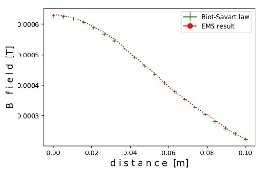
Figure 4 - Comparison of EMS and theoretical results for magnetic flux density along the axis of a toroid

1. Under Results , right click Magnetic flux density in the EMS feature tree
2. Select 3D Vector Plot , Section Clipping .
3. Under Section Clipping tab, select one of the sections that contain the system centerline.
4. Under Vector Options tab, define size, density and shape of the vectors in the plot.                                                                                                                                                                         

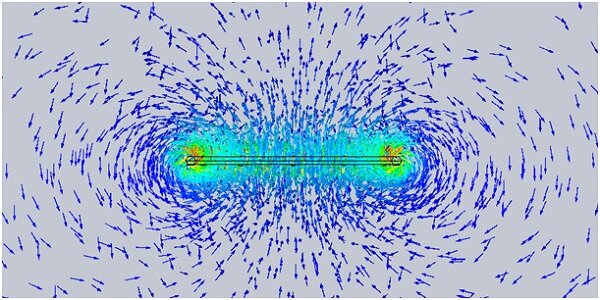
Figure 5 - Section plot of the magnetic flux density

Conclusion