Exploring the Performance of Eddy Current Brakes in Different Applications

What is an eddy current brake?

Eddy currents, generated by electromagnetic induction, occur when electric conductors are exposed to changing magnetic fields or when moving through static ones. Initially seen as problematic due to their heat dissipation, engineers developed methods like laminated materials and cooling systems to mitigate their effects on applications like transformers and motors. Conversely, eddy currents found use in applications such as metal detectors and induction heating. This article explores rotary eddy current brakes, offering frictionless, contactless braking suitable for various industries but with limitations like low torque at low speeds.

Figure 1 - Roller coaster using eddy current retarder

Simulation of the eddy current brakes (ECB)

Engineers and researchers collaborated to develop innovative and robust eddy current brakes. Finite element (FE) solutions have proven more reliable in studying contactless magnetic braking than analytical solutions, which rely on assumptions that may reduce accuracy. EMS, a 3D FEM simulation software from EMWorks Inc., is utilized in this study to analyze rotary eddy current brakes. EMS couples electromagnetic solutions with mechanical analysis to compute magnetic flux, generated eddy currents, braking torque, eddy losses in the rotating disk, angular displacement, velocity, and more.

Two analyses will be conducted during the simulation:

- The first analysis excludes transient mechanical response, focusing on computing torque versus time while the disk rotates at a constant speed.

- The second analysis includes the study of transient mechanical response, computing torque versus time after applying an initial velocity to the rotating disk.

Figures 2a) and 2b) show respectively an isometric and side view of the ECB proposed model. It is made of two non-touched components (separated by air): a rotating copper disk, a fixed arrangement of permanent magnets, and a back iron core (see Figure 3). The remanence of the permanent magnets (NdFeB) is 1.25 T and the relative permeability of the iron core is  . Electrical conductivity of copper is the following:  while it is neglected for the iron material.

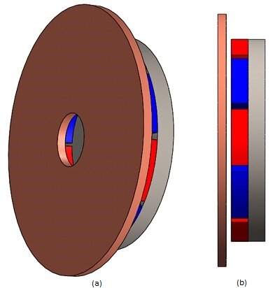
Figure 2 - Eddy current brakes model, a) isometric view b) side view

 

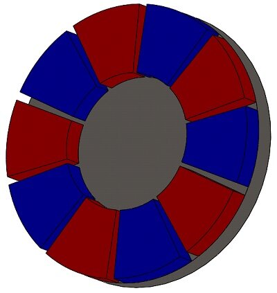
Figure 3 - Arrangement of the permanent magnets and back iron core

Figure 4 depicts a cross-section view of a mesh plot, with mesh elements ranging from 1.3 mm in the copper disk to 10 mm in the iron core. The mesh size can be manually adjusted using the EMS mesher. To effectively capture eddy currents, smaller mesh elements are applied to the disk surfaces. Adjusting the mesh size enables precise analysis and simulation of electromagnetic phenomena within the system.

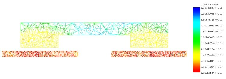
Figure 4 - Cross-section view plot of the mesh

Results and Discussions

Constant Speed 

In this scenario, the disk rotates steadily at 1000 rpm in the counterclockwise direction. Eddy currents induced in the copper disk generate an electromagnetic torque opposing the motion. Figures 5a) and 5b) display fringe and vector plots of the magnetic flux density within the permanent magnets and iron core, respectively. The magnets alternate in direction (+/-) along the axis of the iron core, which serves to minimize magnetic flux losses and align the field with the disk's direction. Additionally, the iron core acts as magnetic shielding, safeguarding equipment like rail sensors and signals from electromagnetic interference. Figure 6 illustrates the H field plot.

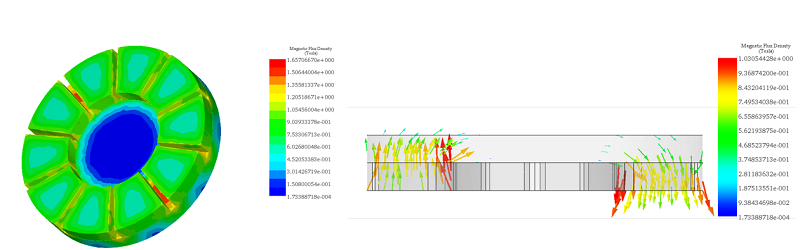
Figure 5 - Magnetic flux density, a) fringe plot, b) vector plot (cross section view)

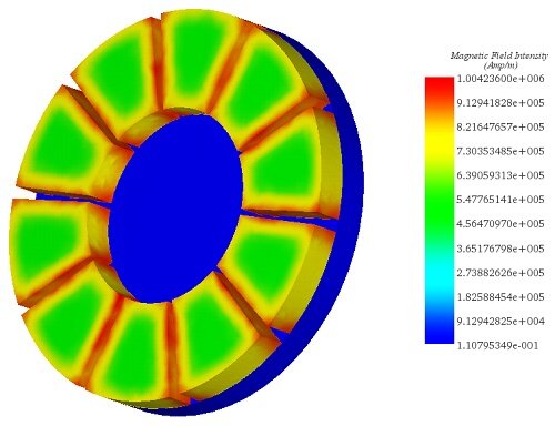
Figure 6 - Magnetic field intensity

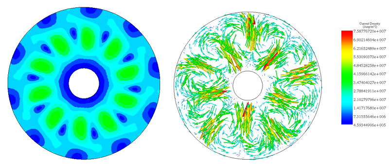
The figures below illustrate the eddy current distribution inside the copper disk. they show several loops of current facing each magnet pole and their directions depend on the magnetization direction of the magnets. The highest induced current is about  . Since the speed is constant, the eddy currents are remaining invariable during the simulation time as shown in the animation in Figure 8.

Figure 7 - Eddy currents, a) fringe plot b) vector plot

 

Figure 8 - Animation of the current distribution

Figure 9 illustrates torque results at different speeds: 500 and 1000 rpm. In both cases, torque remains constant and negative over time, aligning with the disk's positive rotation direction. According to Lenz’s law, eddy currents produce torque opposing the motion. The blue curve represents torque at 500 rpm, while the red curve depicts torque at 1000 rpm. Torque values are lower for the blue curve (10 Nm) compared to the red curve (12.6 Nm), indicating that torque increases with speed. This validates the use of such brakes in high-speed applications, albeit with the caveat of potentially generating more heat in moving parts.

 

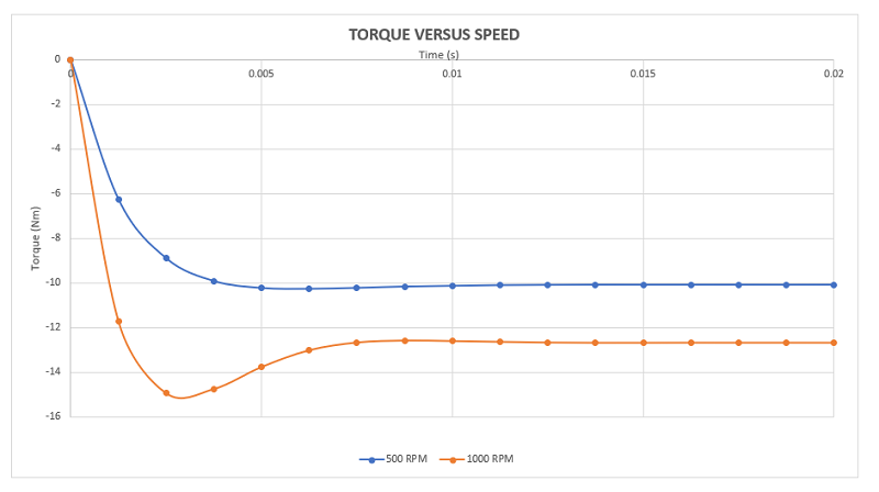
Figure 9 - Generated torque for different speed rate

 

Braking phase

In this section, the braking phase (disk deceleration) is studied. Initially, the disk is rotating with the speed of 1000 rpm, the load torque is suppressed, and the braking torque is applied to slow down the disk. Transient Module of EMS coupled to Motion analysis are used to solve both electromagnetic and mechanical problems. The transient simulation duration is 0.2s. Figure 7 demonstrates plots of the eddy current generated by the rotation of the disk inside a static magnetic field produced by the permanent magnets. Figures 7a) contains the current distribution at 0.005s. The current density peak is around  . This value is measured when the velocity is 1000 rpm. The maximum of eddy current density at 0.05s is about  and the speed is 135 rpm currently step. At speed of 0.35 rpm (0.17s), the average of the current density is very low as shown in Figure 7c). The eddy current density is decreasing from  at the initial angular speed to very low values at speeds close to zero. Hence, this can confirm that the eddy currents are proportional to the speed. Moreover, as can be observed below, the eddy current loops start to disappear when the speed becomes low. 

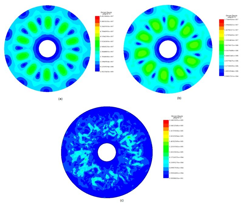
Figure 10 - Eddy current distribution, a) at 0.005s b) at 0.05 c) at 0.17s
 

Figure 11 shows the eddy loss (W) generated by the eddy currents in the spinning disk. Having a behavior identical to the current density, it has a peak of 900W at 0.005s when the speed has its highest value (1000rpm), then it decreases when the disk is decelerating.

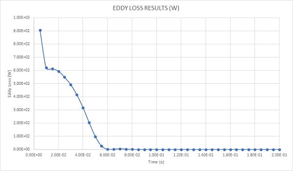
Figure 11 - Eddy loss
 

Figure 12 superimposes the curve of the electromagnetic torque and the disk angular speed. It shows that the torque, generated by eddy currents in the disk, decreases from -3.7 Nm at 0.005s to -2.24Nm at 0.01s, then it increases to reach its highest value around -6 Nm at 0.04s. This can explain the behavior of the disk velocity which drops down from its peak value (1000rpm) at 0.005s until becoming null at 0.057s. Both the angular speed and the torque have opposite directions: the disk is moving in the anti-clockwise direction while the torque has a clockwise direction until 0.57s and reversely from 0.057s to 0.09s (Lenz’s law).

When the speed becomes low, the torque starts to decrease again. After the steady state is achieved (0.1s), both electromagnetic torque and speed are close to zero. This magnetic brake takes 0.057s to stop the disk from rotating.

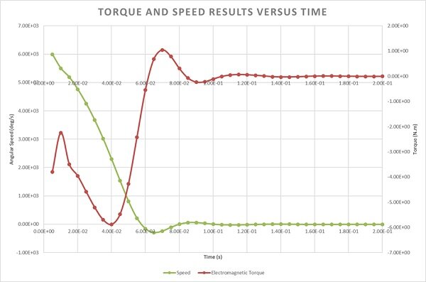
Figure 12 - Braking torque and angular speed curves 
 

Figure 13 presents a comparison of the disk's angular position under two conditions: with and without the eddy current effect. The blue curve depicts the disk's motion when no eddy current is present, meaning no braking torque is applied, and the disk rotates freely. It completes 3.33 revolutions during the 0.2-second simulation. In contrast, the red curve illustrates the angular displacement of the disk with the eddy effect, where braking torque is applied. The disk comes to a halt at 0.57 seconds after rotating 161 degrees.

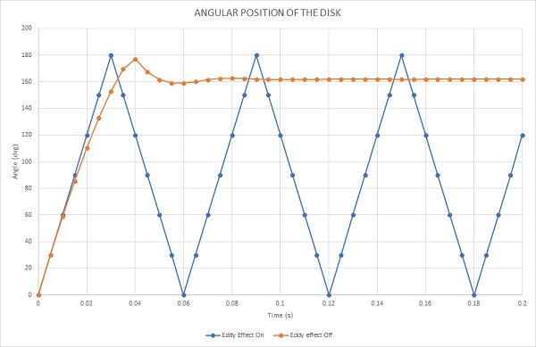
Figure 13 - Angular displacement of the disk
 

Figure 14 contains an animation of the eddy current distribution during the deceleration phase of the disk. It illustrates the diminution of the current with the speed.

Figure 14 - Eddy currents versus time during the braking phase

 

Conclusion

This comprehensive guide delves into the analysis and understanding of eddy current brakes, offering insights into their performance across various applications. Armed with this knowledge, engineers and researchers can make informed decisions when designing and implementing eddy current braking systems.

References

[1]: Kerem Karakoc , Afzal Sulemana , Edward J. Park. Analytical modeling of eddy current brakes with the application of time varying magnetic fields. Applied Mathematical Modelling 000 (2015) 1–12