Performance Analysis of Synchronous Generator Performance under Different Loads

Synchronous Generators

This application note explores the performance of a typical synchronous generator used in aircraft electrical systems under varying load conditions. Utilizing EMWorks 2D software's finite element method (FEM) tool, the generator's behavior is analyzed with resistive, inductive, and capacitive loads, comparing parameters such as load current, back EMF, and terminal voltage.

Case Study

The study utilizes a salient pole synchronous generator with 10 rotor poles and 30 stator slots, as depicted in Figure 1. Its stator slot features a double-layer winding configuration with a winding factor of 0.866. Parameters of the generator are outlined in Table I. Notably, aircraft applications necessitate smaller and higher frequency machines, thus the base speed of the studied machine is set at 12000 rpm.

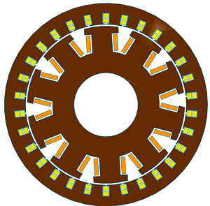
Figure 1. A 2-D Cross-Section View of the Synchronous Generator Under Study

Table I: Synchronous Machine Parameters

Mechanical Speed (rpm)	12000
Rated Power (kVA)	200
Output Voltage (V)	115
Rated Current (A)	577
Rotor Excitation DC Current (A)	180
Stator and Rotor Core Material	M27

Comparative Analysis and Results

In this section, the synchronous generator under three different load conditions is simulated. In all cases, the impedance magnitude of the load is kept equal to 10 , while the load angle is varied to achieve the power factor of 1 (unity), 0.65 leading and 0.65 lagging. A balanced three-phase load with a star connection is considered for all the load conditions and the simulation is performed using the EMWorks 2D software. The DC excitation of the rotor is equal to 180 A and the rotor mechanical speed is equal to 12000 rpm for all the conditions. Based on the following equations, the resistance, inductance, and capacitance values are calculated and used in the simulations. Table II summarizes the different load types and the corresponding inputs of each study. Figure 2 shows one example of the synchronous generator connected at 0.65 lagging load.

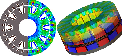
Figure 3 shows the magnetic flux density plot of the synchronous generator connected to a purely resistive load at t = 0.5 ms. As observed from the plot, the rotor poles get saturated at this instance and the magnitude of magnetic flux density is approximately equal to 2.12 T. A similar flux distribution plot can be obtained for the other load conditions.

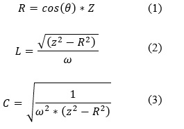
Table II: Load Summary

Case	Load Power Factor	R ()	L (mH)	C (mF)	Load Angle
1	1 (unity)	10	0	0	0°
2	0.65 lagging	6.43	1.22	0	50°
3	0.65 lagging	6.43	0	0.02078	-50°

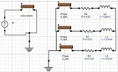
Figure 2. Modelled Circuit Schematic of the Synchronous Generator at 0.65 Lagging Load

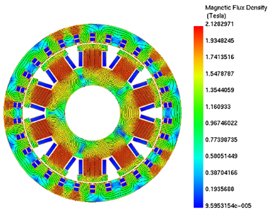
Figure 3. Magnetic Flux Density Distribution of a Synchronous Generator at Purely Resistive Load

In this section current and voltage, waveforms are plotted vs. time for each case. It can be observed that the currents are shifted from voltage due to the difference in the load angle. Figure 4 represents case 1 results with a purely resistive load, it can be observed that the current and voltage are in phase with each other. Figure 5 represents case 2 results with RL load, here voltage leads with the current. Similarly, Figure 6 represents case 3 results with RC load where voltage lags with the current

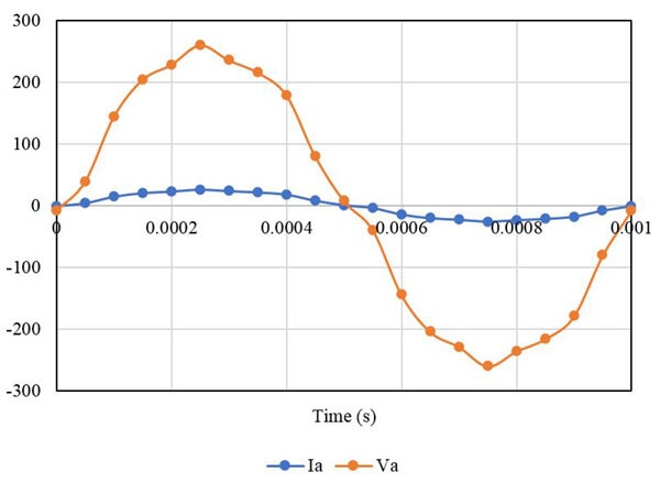
Figure 4. Output Current and Voltage Waveforms with the Purely Resistive Load

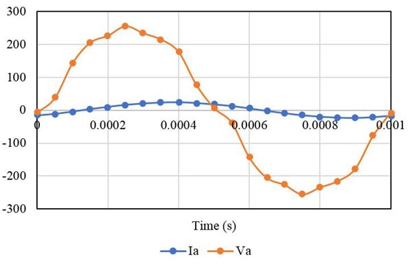
Figure 5. Output Current and Voltage Waveforms with the RL Load

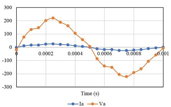
Figure 6. Output Current and Voltage Waveforms with the RC Load

Table III: Output Current and Voltage Amplitudes Comparison for Different Types of Load

Load Types	Maximum		RMS
Load Types	Current	Voltage	Current	Voltage
R	25.97 A	259.7 V	18 A	180 V
RL	24 A	255.3 V	16.6 V	178.6 V
RC	25 A	219.5 V	16.7 A	146.8 V

Referring to Table III, it can be inferred that the maximum current is obtained by a purely resistive load whereas the minimum current is performed by the RL load. Moreover, the difference between the magnitude of the output current obtained among all the cases is small as their impedance magnitude is equal.

Figure 7 represents the output three-phase back EMF waveforms of the synchronous generator. The back EMF voltage is obtained by supplying the rotor excitation current and the armature winding circuit is kept open as shown in Figure 8. The back EMF waveform remains the same for the three loads. Fig 9,10 and 11 present the back EMF produced by the generator at different speeds, excitation currents, and the number of turns of the rotor winding. Fig 9 confirms that the generated power has a linear behavior regarding the speed.

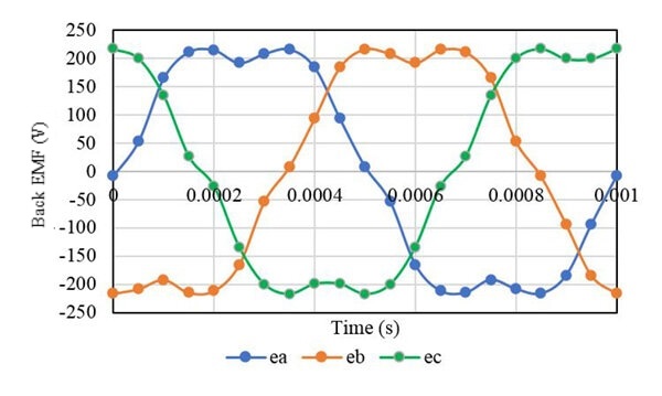
Figure 7. Back EMF Waveforms

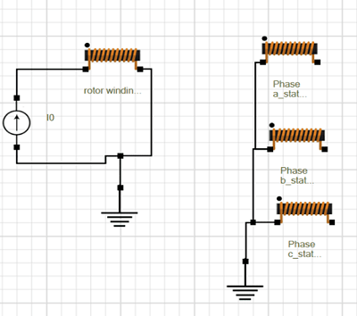
Figure 8. Open Circuit Schematic for Back EMF Simulation

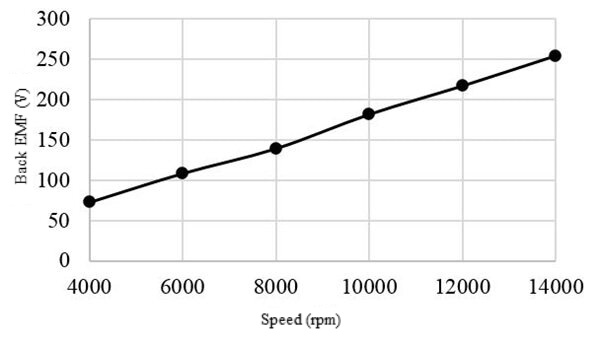
Figure 9. Back EMF vs. Speed

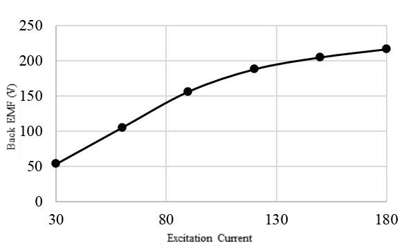
Figure 10. Back EMF vs. Excitation Current

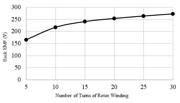
Figure 11. Back EMF vs. the Number of Turns of the Rotor Winding

Conclusion

In this application note, three different types of load such as pure resistive, RL, and RC load keeping the same impedance are compared for synchronous generators. The electromagnetic performances such as output current, output voltage, and the back EMF are obtained using the EMWORKS 2D software. It has been found that the load angle affects the phase delay between the output current and voltage waveform. Also, the back EMF at different speeds and excitation current values are simulated and analyzed.

References

[1] Wildi, Theodore. Electrical Machines, Drives and Power Systems. 6th ed. Upper Saddle River: Pearson Practice Hall, 2006. 377-396 (Wildi, 2006)

Share on