

Inductive Proximity Sensor
The inductive sensor detects target position by measuring PCB coil inductance changes. EMS calculates coil inductance at different target positions, aiding circuit design for accurate measurement systems.
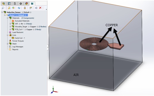
CAD model of an Inductive Proximity Sensor
Inductive sensors, commonly used for position detection, employ a coil excited by high-frequency AC current. Operating on Faraday's law of induction, these sensors measure coil inductance changes to detect targets. In the absence of a target (Figure 1), the coil's inductance is known and computable via EMS. However, when a conductor target is present directly above the coil (Figure 2), the coil's inductance alters, allowing the sensor to identify the target's presence. Notably, inductive sensors exclusively function with conductive targets.
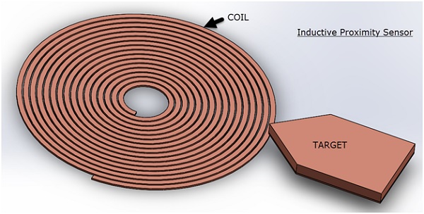 Figure 1 - Target not in the direct proximity
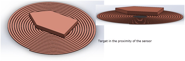
Figure 2 - Target directly above the sensor
EM Simulation of the Inductive Proximity Sensor
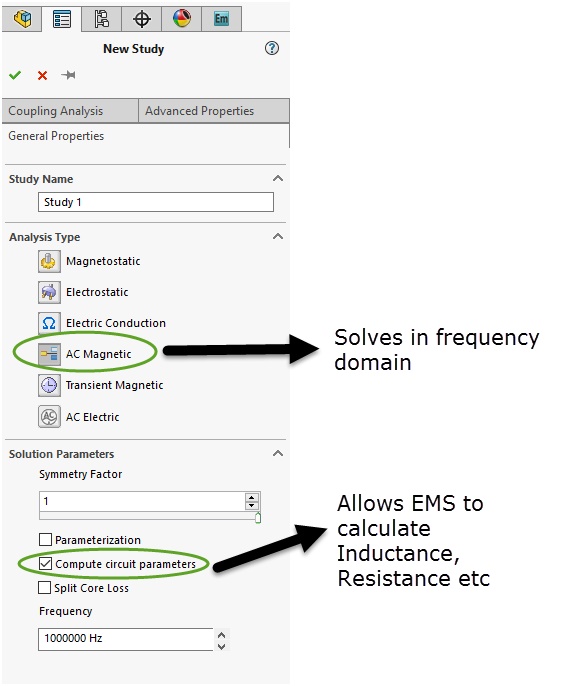
EMS analyzes these sensors through AC Magnetic simulation, solving problems in the frequency domain. Outputs include coil inductance, resistance, magnetic flux density, field intensity, and eddy current density. As the solution is frequency-based, field quantities are provided as functions of phase angle. In the depicted simulation (Figure 3), the AC Magnetic study's frequency was set at 1 MHz, with EMS capable of resolving frequencies up to several hundred megahertz. This comprehensive analysis enables engineers to understand sensor performance across a range of frequencies, aiding in the design and optimization of inductive sensors for various applications.
Coil
The coil is represented as a Solid Coil, with a current of 1 mA flowing as depicted in Figure 4. EMS offers modeling options for both Solid and Stranded coil configurations, with Solid coil accounting for eddy currents. However, in this simulation, eddy currents within the coil are disregarded. Nonetheless, eddy effects are factored in for the movable target material, constructed from copper. This selective approach allows for a focused analysis of the target's response to the inductive sensor while simplifying the model for efficient computation and accurate assessment of sensor behavior.
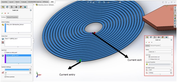 Figure 4 - Current direction in the Solid coil
Materials
In this simulation, three components are considered: the coil and the target, both constructed from Copper, and the Air region, represented as Air. Figure 5 illustrates the modeled components for this simulation. The Air region plays a vital role in electromagnetic simulations conducted with EMS, facilitating the computation of field quantities within the airspace surrounding the coil and the target. EMS boasts a comprehensive material library, offering customization options and featuring a wide array of commonly utilized materials in Electrical Engineering applications. This extensive library enhances versatility and accuracy in modeling various electromagnetic phenomena.
Mesh
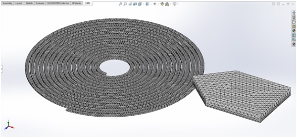
EMS includes a fully automatic mesh generator that accurately captures the geometry from your CAD system, eliminating the need for any modifications to your CAD geometry. To ensure precision and capture the skin depth in the target, a mesh control is applied specifically to the target region. This feature enables users to define mesh sizes for selected areas within the model. Figure 6 illustrates the mesh generated by EMS, showcasing its capability to efficiently handle complex geometries and ensure accurate simulation results.
Inductance change calculation
The Results section is divided into 3 parts –- Inductance calculation of the coil
- Resistance calculation of the coil
- Field plots (Magnetic flux density, Magnetic field intensity, eddy currents in the target etc)
Inductance
The coil inductance serves as a crucial parameter for circuit design, aiding engineers in developing motion detection systems. Figure 7 presents a table showcasing the coil inductance at two distinct positions: when the target approaches the coil but remains distant, and when the target directly overlaps the coil. The inductance decreases from 1.27 micro Henry to 1.07 micro Henry when the target enters the coil's vicinity, marking a 15.7% reduction. These precise values enable engineers to design circuits with ample sensitivity to detect such variations, facilitating efficient motion detection and response mechanisms.
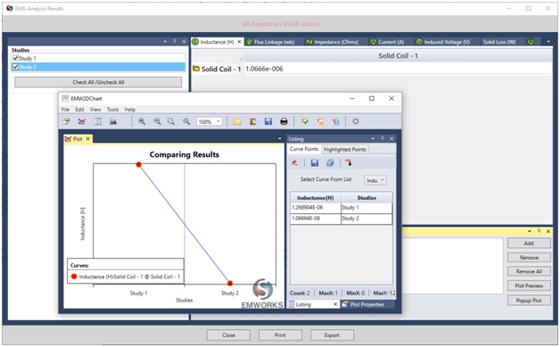 Figure 7- Inductance comparison between the 2 positions
Resistance
The coil's resistance remains constant regardless of the target's position, representing an intrinsic property of the coil. EMS accurately calculates the coil's resistance, accounting for its precise geometry. Figure 8 illustrates the computed coil resistance, determined to be 0.35 Ohms. It's essential to note that this resistance value signifies the DC resistance of the coil, serving as a fundamental parameter for circuit analysis and ensuring stable operation across various conditions.
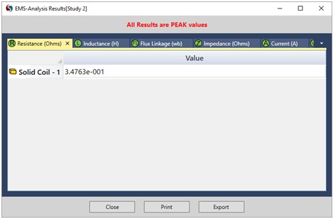 Figure 8- EMS computes the DC resistance of the coil
3D fields generated by an Inductive Proximity Sensor
Figures 9 and 10 illustrate the magnetic field density and intensity plots corresponding to position 2, when the target is in proximity to the coil. Observe that in the magnetic flux density vector plots, the vectors passing through the target appear smaller due to the induced eddy currents on the target. These eddy currents counteract the field generated by the coil. EMS offers versatile visualization tools including 3D plots, vector plots, and section plots, aiding in a comprehensive understanding of field behavior in different scenarios. These visualizations are invaluable for engineers in optimizing sensor performance and refining design parameters.
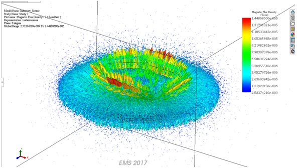 Figure 9- Vector plot of the magnetic flux density
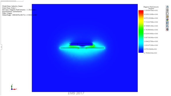 Figure 10- Section plot of the Magnetic Field Intensity
Figure 11 shows the distribution of the eddy currents in the target when it is in the proximity of the sensor (or the coil). Notice how the vectors of the current create a flux that opposes the flux created by the coil.
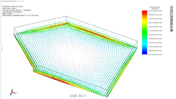
Figure 11- Eddy currents in the target