

Multiphysics simulation using EMS
EMS facilitates multi-physics simulations through its ability to couple magneto-mechanical fields. This example demonstrates EMS's utility in assessing the impact of a steady magnetic field on the geometry of Silicon steel RM50, a material with high saturation levels. Two distinct current densities are applied across two different regimes, enabling a comprehensive analysis. The coupling mechanism involves transferring the magnetic force acting on the rectangular workpiece to the mechanical solver, ensuring a seamless integration of magnetic and mechanical aspects in the simulation process.
Problem description
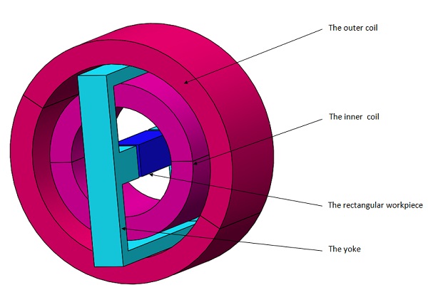
The magnetic system depicted below comprises two concentric coils supplied with constant current and a ferromagnetic yoke enveloping a rectangular test body. This model seeks to analyze the mechanical deformation of the test body under both linear and saturation regimes of the ferromagnetic material within the yoke and test body. Two distinct current densities are applied to assess body deformation.
Simulation Setup
To establish a Magnetostatic Study coupled with Structural Analysis in EMS, adhere to these crucial steps:
- 1. Assign appropriate materials to all solid bodies.
- 2. Implement essential electromagnetic inputs.
- 3. Apply required structural inputs.
- 4. Mesh the complete model.
- 5. Initiate the solver for computation.
Materials
Electromagnetic equations are solved across the entire solution domain, while stress analysis is confined to the rectangular workpiece.
Table 1 - Material properties
|
Material |
Relative Permeability |
Electrical Conductivity (Mho/m) |
Elastic modulus (Pa) |
Poisson's Ratio |
|
Copper |
1 |
5.9980e+07 |
Not required |
Not required |
|
Air |
1 |
0 |
Not required |
Not required |
|
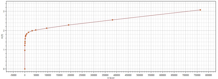
Silicon steel (RM50) |
* 2175 (Linear case) * BH curve (nonlinear case) |
2.1186e+06 |
2.035e+011 |
0.285 |
Electromagnetic inputs
In this study, two wound coils are defined as the current source of the problem.
Table 2 - Coil information
|
Number of turns |
Wire diameter (mm) |
Current amplitude (A) |
||
|
Wound Coil 1 |
1 |
0.91168568 mm |
47336.25 for case 1 473362.5 for case 2 |
|
|
Wound Coil 2 |
1 |
0.91168568 mm |
4887.5 for case 1 48875 for case 2 |
|
Mechanical boundary conditions
Fixed constraint on four edges of the rectangular workpiece (highlighted below in Figure 3)
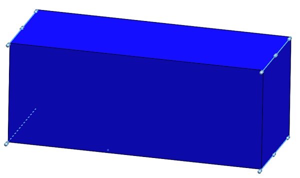
Figure 3 - Fixed constraint applied on the model edges
Meshing
Meshing is critical in design analysis, with EMS determining an appropriate element size based on the model's volume, surface area, and geometric details. The mesh size, defined by nodes and elements, depends on factors like geometry, dimensions, and mesh control settings. Opting for a larger element size in early design stages can expedite solutions when approximate results suffice. Conversely, for higher accuracy, a smaller element size is necessary. Balancing these factors ensures an efficient mesh for accurate simulations without sacrificing computational speed.
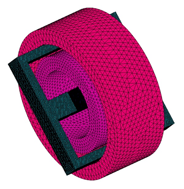 Figure 4 - Meshed model
Magneto-mechanical results
Figure 5 depicts a 3D plot of magnetic flux across the entire magnetic system, illustrating the nonlinearity of permeabilities in both the test body and the yoke under the second applied current.
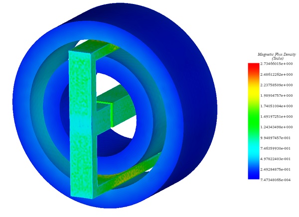
Figure 5 - Magnetic flux plot
Figure 6 presents the current density distribution in the two coils, for the second treated case of current density.
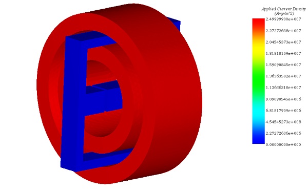
Figure 6 - Current density plot
Figure 7 shows the mechanical deformation of the rectangular 3D test body under the second applied current density when permeabilities of the yoke and the test body are nonlinear.
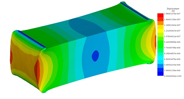
Figure 7 - Resultant displacement plot
Table 3 - Deflection of the workpiece under the two used current densities, using two different permeabilities
| Current density | Linear permeability | Nonlinear permeability |
| J=2.5e+06 A/m^2 | 0.98 | 0.88 |
| J=25e+06 A/m^2 | 87.94 | 5.65 |
EMS emerges as a powerful tool for examining the intricate interplay between magnetic fields and mechanical systems. Through this application note, we've unveiled EMS's capability to seamlessly couple magneto-mechanical fields, offering valuable insights into material behavior and system optimization. As industries push boundaries, understanding and harnessing this coupling mechanism become increasingly crucial for engineering innovation. Leveraging EMS's capabilities empowers engineers to delve deeper into Multiphysics phenomena, driving advancements and unlocking new possibilities across diverse domains.
Reference
[1]:Se-Hee Lee, Xiaowei He, Do Kyung Kim, Shihab Elborai, Hong-Soon Choi, II-Han Park and Markus Zhan.2005. Evaluation of the mechanical deformation in incompressible linear and nonlinear magnetic materials using various electromagnetic force density methods. Journal of applied physics. Volume 97, Issue 10