

Voice Coil Actuator
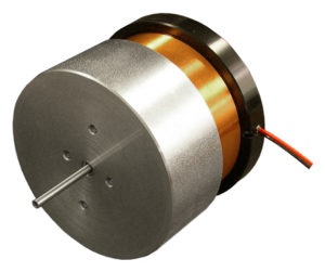
The voice coil actuator, utilizing Lorentz force, offers precise small-scale positioning. Also known as a non-commutated DC linear actuator, it's easy to control, fast, and compact. This makes it a superior alternative to traditional electric motors, ideal for applications requiring precise positioning. With capabilities spanning from 10nm to 100mm, it excels in nano- and micro-positioning tasks. Learn more about its optimal applications - at https://www.linearmotiontips.com/when-are-voice-coil-actuators-best-linear-motion-option/
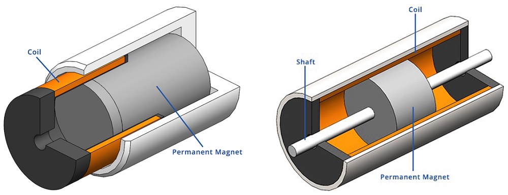
The voice coil actuator primarily consists of a permanent magnet and a stranded coil winding, with additional ferromagnetic components sometimes incorporated for enhanced efficiency. In this actuator, either the coil or the permanent magnet can serve as the moving component. Figures 2 and 3 depict two common configurations: moving coil and moving permanent magnet, respectively. The conversion of electrical energy into mechanical motion follows the Lorentz force principle, stating that when a conductor carrying a current is placed in a magnetic field, an orthogonal electromagnetic force is generated. This force's magnitude is determined by the formula: (F = J imes B), where (J) represents current density within the conductor and (B) signifies the magnetic field.
Voice coil actuators find widespread use across various industries. In the medical sector, they feature portable ventilators, metering, and dosing pumps, among other applications. Similarly, industries such as semiconductors and electronics leverage voice coil actuators for mounting, assembling, and product testing, thanks to their exceptional displacement resolution. Additionally, their low inertia makes them ideal for auto-focusing motor actuators in smartphone cameras and other compact applications.
Voice Coil actuator Vs Solenoid Actuator
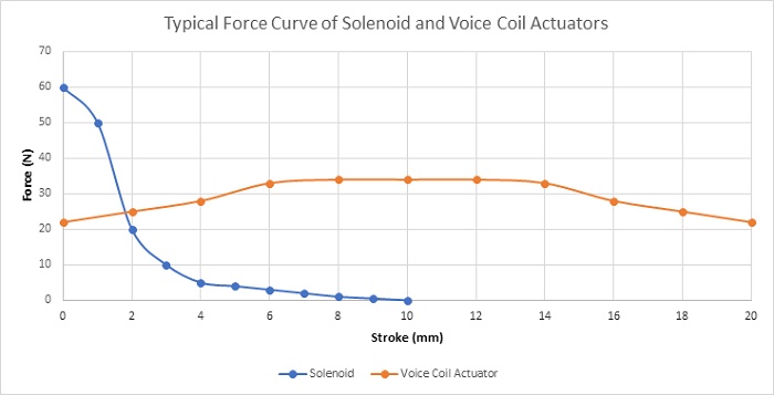
The table below and Figure 3 provide a comparative analysis of the key characteristics and typical force behaviors between voice coil and solenoid actuators. While solenoids offer higher force density within a limited stroke range, voice coil actuators are capable of generating a consistent, albeit lower, force across a wider stroke range. Additionally, voice coil actuators typically deliver more robust and controllable force output.
| Voice Coil Actuator | Solenoid Actuator | |
| Stroke | Up to 5 inches | ¼ inches |
| Force | Low | High |
| Constant Force | Yes | No |
| Reversible | Yes | No |
| Position/ Force Control | Yes | No |
| Cost | Moderate | Low |
Problem description
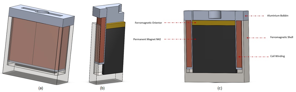
In this article, we delve into the study of a voice coil actuator [3]. Utilizing optimal actuator parameters determined in previous research [3], a series of simulations will be conducted. The initial section focuses on static analysis to compute the Lorentz force of the coil concerning both current and actuator positions. Subsequently, transient magnetic studies will explore current variations under different DC voltage excitations. Simulation outcomes will be compared with experimental data from [3]. Electrodynamic simulation will then be employed to calculate mechanical output parameters such as linear displacement, speed, and acceleration. Additionally, an electrothermal analysis will examine the temperature evolution of the voice coil actuator. Leveraging EMS, various simulations will be conducted on the voice coil actuator. Figures 4a), 4b), and 4c) depict comprehensive and cross-sectional views of the examined voice coil device. Featuring a stranded copper coil with 760 turns, the actuator moves axially within the airgap zone between the ferromagnetic shell and the stationary, axially magnetized neodymium permanent magnet N42. Both the orientor and shell consist of soft iron renowned for its high permeability, facilitating efficient magnetic circuit paths. The flux orientor further aids in field guidance. A supporting bobbin is inserted to stabilize the coil.
Simulation and Results
Static Simulation -Geometrical Parametric Sweep
The initial simulations involve varying DC current rates while adjusting the positions of the moving components (coil and bobbin). A parametric sweep study is set up to analyze magnetic flux, Lorentz force, and coil parameters. Figures 5a) and 5b) present full and cross-sectional views of magnetic flux density plots at +10A current, with the coil and bobbin positioned 10mm apart. The average magnetic flux ranges between 1.3T and 1.74 T. Front and side cross-section views of magnetic field vector plots are depicted in Figures 6a) and 6b). The coil's current density is measured at 1e8A/m^2.
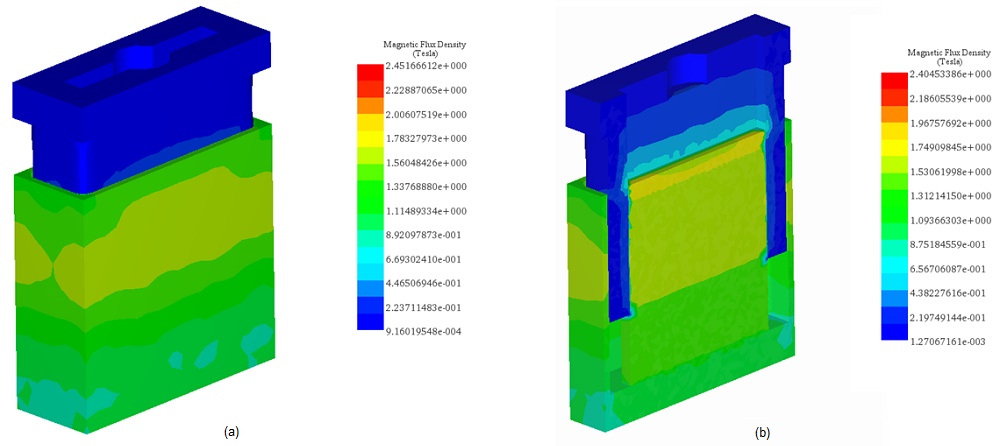
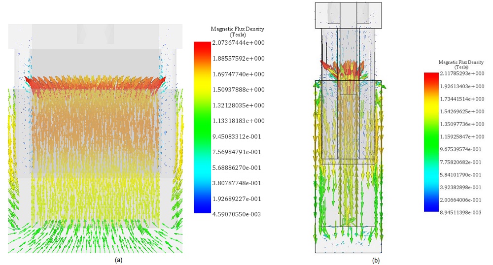
Figure 7 illustrates the comparison between experimental [3] and simulation results of the Lorentz force across various DC currents and stroke values. The maximum force (approximately 33N) occurs with a current of -10A at a position of 10mm. Force values measured between 4mm to 16mm stroke remain relatively constant across different applied current rates, offering consistent force rates with larger strokes for enhanced acceleration. Figure 8 displays a plot of force peak values for different currents, showcasing a proportional linear relationship with current, and highlighting the actuator's simple and flexible force control.
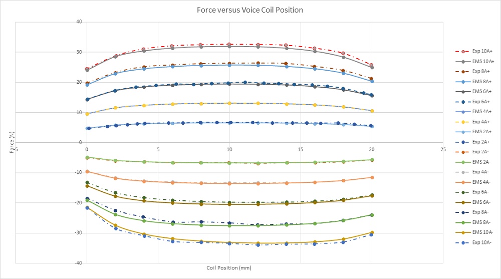
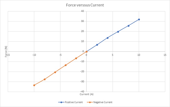
Figure 9 illustrates the force sensitivity parameter for various input currents across the stroke. This parameter remains constant with respect to the current and is solely dependent on the coil position. The simulated average value of the force sensitivity parameter, computed by EMS, is approximately 3.2N/amp, closely matching the experimental measurement of 3.1N/amp. This agreement underscores the accuracy of the simulation results in predicting the force sensitivity of the actuator.
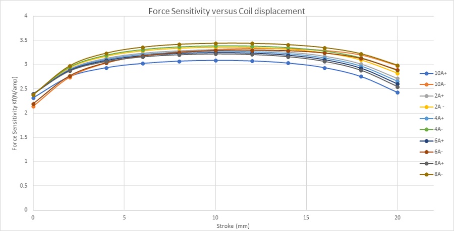
Figure 10 depicts the inductance curve plotted against coil displacement. The inductance gradually decreases from 5mH at 0mm to 4.48mH at 20mm. Despite this variation, the change is negligible, allowing us to treat the coil inductance as constant throughout the stroke. This consistency simplifies the analysis and facilitates the design of control systems for the voice coil actuator, as it ensures predictable behavior across different displacement levels.
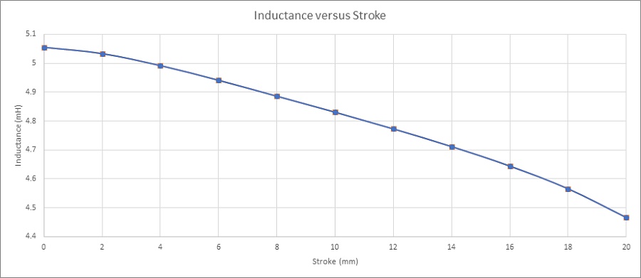
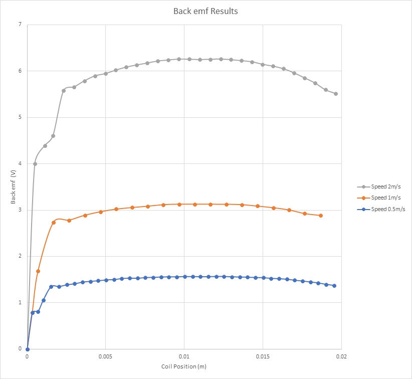
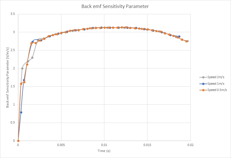
Figure 11 illustrates the Back EMF results of the coil across various velocities plotted against the center of mass of the moving components. The graph reveals a direct correlation between Back EMF and speed, with a peak of 6.25V achieved at a speed of 2m/s. Meanwhile, Figure 12 presents the computed Back EMF sensitivity parameter (V/speed) relative to coil position. Notably, this parameter remains constant regardless of coil speed, averaging at 3.1 V/m/s.
| EMS | Experimental | |
| Current | +10 A | +10A |
| Resistance | 20.35 | 20.5 |
| Inductance | 5mH | 5mH |
| Maximum Generated Force | 34N | 33.4N |
| Force Sensitivity Parameter | 3.2N/amp | 3.1N/amp |
| Back emf Sensitivity Parameter | 3.1V/m/s | 3.1V/m/s |
Transient Simulation using EMS – Current and force calculation for different voltages
In this section, electromagnetic simulation is conducted using the Transient module of EMS. The coil is energized with varying DC voltages, allowing for the computation of magnetic fields, current, and Lorentz force. Figure 13 depicts the magnetic flux density once the system reaches a steady state.
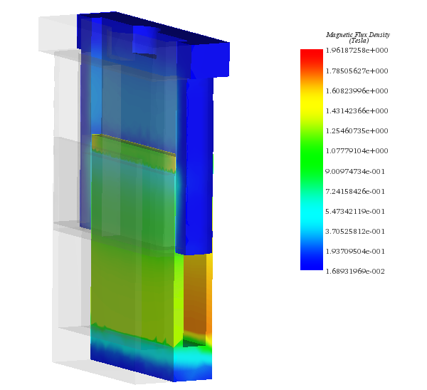
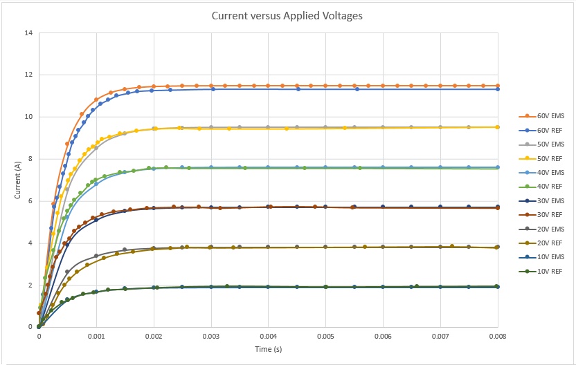
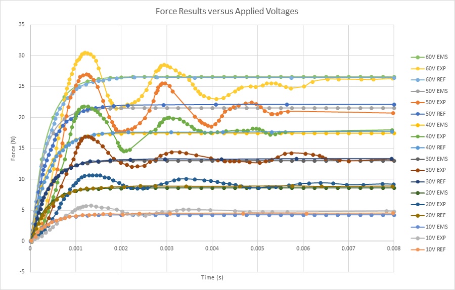
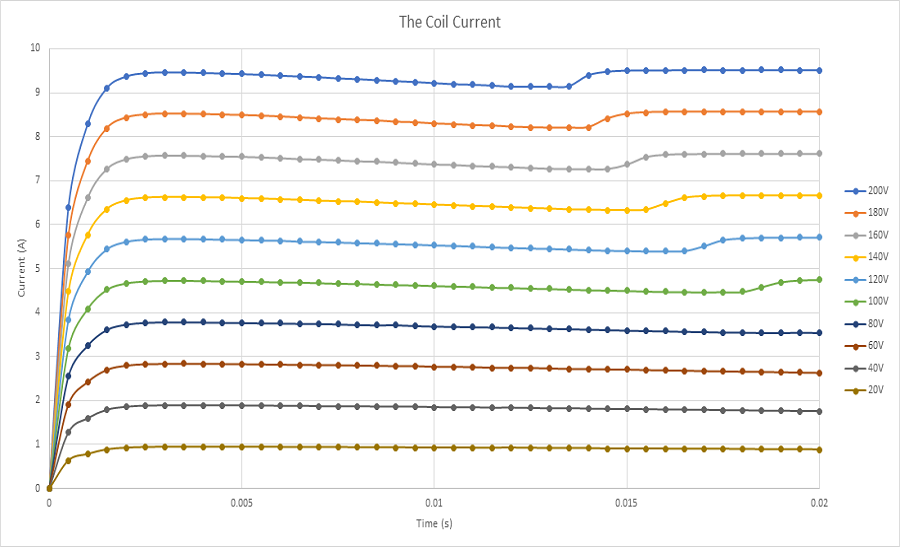
Figure 14 depicts the current response calculated for various applied voltage rates, showcasing the achievement of a steady state within 2ms. This quick stabilization enhances the system's time response. At 10V and 60V applied to the stranded coil, the computed currents are 2A and 11A, respectively. Figure 15 presents force results at a static position of 12mm. Experimental tests show some oscillations before settling into a steady state. With a 10V DC voltage, a force of 4.5N is attained, while it reaches 26N with a 60V voltage, indicating a direct relationship between voltage and force.
Electro-mechanical simulations are conducted using EMS coupled with motion analysis to compute various outcomes such as magnetic fields, current, coil displacement, speed, and acceleration. Neglecting eddy current effects due to motion, these simulations reveal critical insights. Figure 16a) displays magnetic flux density at 20ms and 20V, showing a peak field strength of 1.77T concentrated at the iron shell's thin walls. At 20ms, the coil registers 0.88A current and a 4.78mm displacement. In Figure 16b), magnetic flux at 9ms and 200V reveals peak values of approximately 2T within the iron shell, with the coil positioned at 8.6mm and a current of 9.26A. Animated magnetic field depictions are presented in Figures 17a) and 17b).
-in%20case-of-20V-b)in-case-of-200V.jpg)
%20.gif)
(a)
.gif)
(b)
Figures 18a), 18b), and 18c) depict the linear displacement, speed, and acceleration of the coil under various applied voltages. At 20V DC voltage, the coil moves from 0 mm at 0s to 4.7mm at 20ms, achieving a maximum speed of nearly 0.5 m/s and an acceleration of about 30 m/s^2. With a 200V DC voltage, the coil extends from 0 mm to 20 mm in 13ms, resulting in a maximum speed and acceleration of 3.3 m/s and 308 m/s^2, respectively. Currents in the coil measure 9.5A and 0.9A for applied voltages of 200V and 20V, respectively. The relationship between voltage and speed is elucidated in Figure 19, where Lorentz force, directly proportional to current, increases with applied voltage.
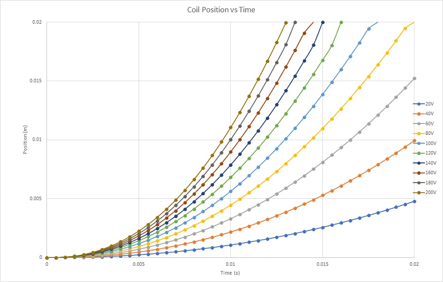
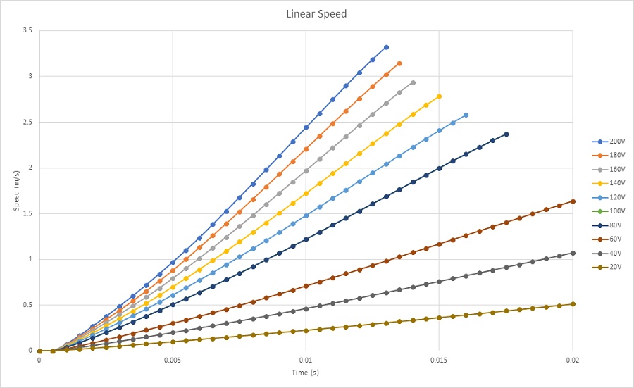
Figure 18b - Coil speed
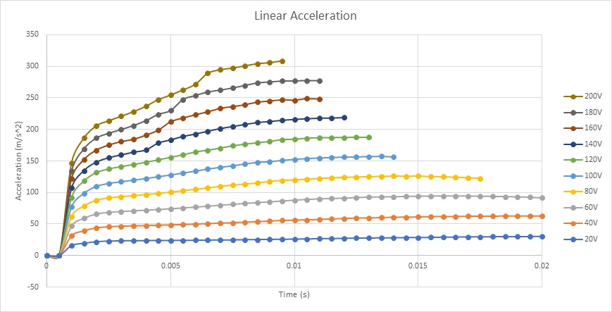
Figure 18c - Coil acceleration
Electrothermal Analysis – Winding loss and temperature calculation of the voice coil actuator
This analysis focuses on electromagnetic losses and the resultant temperature increase in the voice coil actuator. With eddy currents disregarded, copper losses (winding losses) constitute the primary electromagnetic losses. As per the Joule law, current flow through the winding conductors generates Joule heat, leading to a proportional rise in the actuator's temperature.
Transient electrothermal analysis, conducted using EMS, calculates winding losses and the temperature evolution over time for a stationary coil position. EMS facilitates thermal coupling analysis seamlessly. Given the significantly smaller electromagnetic time constant compared to the thermal time constant, achieving a steady state in an electromagnetic solution occurs rapidly, whereas attaining a steady state in thermal analysis requires a longer duration. Thus, employing various simulation end times and time step sizes expedites the analysis.
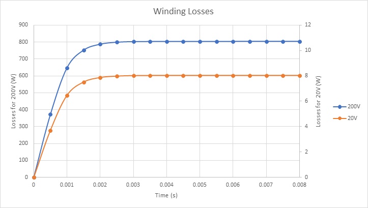
Figure 20 illustrates the winding loss outcomes for two voltage scenarios. At 200V and 20V DC voltages, copper losses in the voice coil amount to approximately 800W and 8W, respectively.
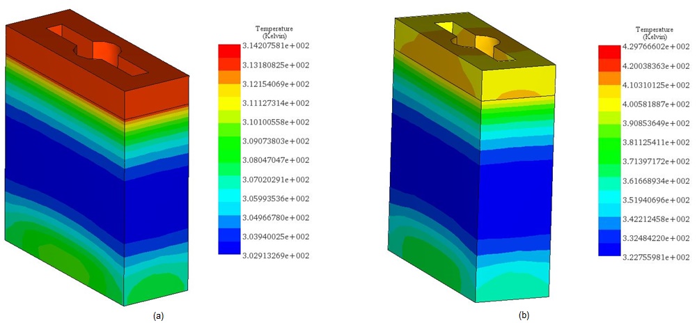
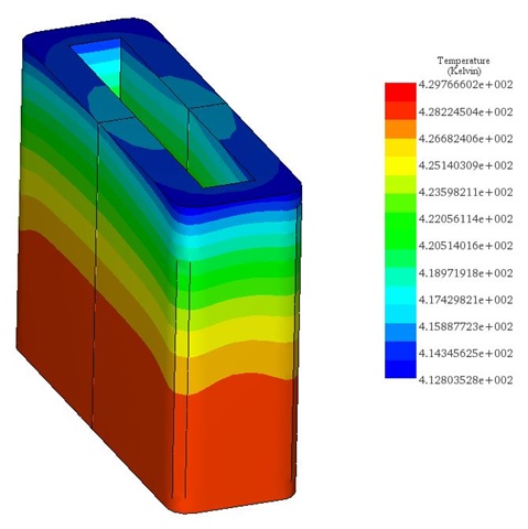
Figures 21a) and 21b) depict the final temperature distribution within the voice coil actuator for 20V and 200V, respectively. The heat generated inside the coil, attributed to copper losses, subsequently diffuses throughout the entire system via conduction.
In the 20V scenario, the temperature peaks at 314 K after 60 seconds, while in the 200V case, it climbs from the ambient temperature of 300 K to 429 K within 5 seconds, as evidenced in Figure 22. This emphasizes the coil's role as the primary heat source. The temperature evolution across the entire system is illustrated in Figure 23.
In conclusion, the detailed exploration of voice coil actuators reveals their remarkable capabilities and versatility across multiple industries. By comparing their advantages with other linear motion options, this study underscores their potential for precision and efficiency. The alignment between simulation and experimental results signifies a promising avenue for further advancements in actuator technology. With a clearer understanding of their benefits and applications, future developments can leverage voice coil actuators for enhanced performance and cost-effectiveness.
References
[1]: https://www.linearmotiontips.com/when-are-voice-coil-actuators-best-linear-motion-option/
[2]: https://www.machinedesign.com/mechanical-motion-systems/article/21836669/what-is-a-voice-coil-actuator
[3]: Vahid Mashatan. Design and Development of an Actuation System for the Synchronized Segmentally Interchanging Pulley Transmission System (SSIPTS). Department of Mechanical and Industrial Engineering University of Toronto 2013