Heben Sie das Design elektromechanischer Systeme mit EMWorks auf und gewährleisten Sie Präzision und Effizienz bei Aktuatoren und Solenoiden.

Revolutionieren Sie das Design von Antennen und Radomen mit der elektromagnetischen Simulation von EMWorks für überlegene Konnektivität und Schutz.
Innovieren Sie im Bereich der biomedizinischen Technik mit EMWorks, optimieren Sie medizinische Geräte und untersuchen Sie die Auswirkungen von EM-Exposition.
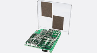
Revolutionieren Sie die elektronische Konstruktion mit den EDA-Tools von EMWorks, optimieren Sie Leiterplatten, EMC und HF-Komponenten für überlegene Leistung.
Revolutionieren Sie elektromechanische Designs mit EMWorks und beherrschen Sie die Komplexitäten elektrischer Maschinen und Antriebe.

Fördern Sie die Elektrofahrzeugtechnologie mit den Simulationen von EMWorks für die Motorentwicklung, Ladesysteme und EMC.
Meistern Sie EMI- und EMC-Herausforderungen mit EMWorks und verbessern Sie die Sicherheit und Leistung von Geräten in verschiedenen Branchen.

Optimieren Sie Ihre HF- und Mikrowellenkomponenten mit den ausgefeilten Simulationstechnologien von EMWorks für eine verbesserte Leistung.
Optimieren Sie magnetische Felder mit EMWorks für Magneten und Arrays, um die Leistung in verschiedenen Anwendungen zu verbessern.
Erleben Sie integrierte Mehrphysik-Simulationen durch die Kopplung von elektromagnetischen, thermischen und strukturellen Analysen.
Innovieren Sie im Bereich der zerstörungsfreien Prüfung mit den fortschrittlichen Sensoren und NDT/NDE-Lösungen von EMWorks in verschiedenen Branchen.

Innovieren Sie im Bereich der Energieingenieurwissenschaften mit EMWorks. Entwerfen Sie effiziente Transformatoren und Hochspannungskomponenten.